Note
Go to the end to download the full example code
Concave penalties#
This example considers proximal operators of concave separable penalties.
import matplotlib.pyplot as plt
import numpy as np

import pyproximal

plt.close('all')
x = np.linspace(-5, 5, 101)


def compare_penalty_and_proximal_operator(penalty):
    fig, ax = plt.subplots(1, 2)
    ax[0].plot(x, penalty.elementwise(x), label=penalty.__class__.__name__)
    ax[0].plot(x, np.abs(x), 'k--', label='l1')
    ax[0].set_aspect(2)
    ax[0].set_xlim(-5, 5)
    ax[0].set_ylim(0, 5)
    ax[0].set_title('Penalty')
    ax[0].legend(loc='upper center')
    for tau in [0.25, 0.50, 0.75, 1.00]:
        ax[1].plot(x, penalty.prox(x, tau), label=f'tau={tau:.2f}')
    ax[1].plot(x, x, 'k--')
    ax[1].set_aspect('equal', 'box')
    ax[1].set_xlim(-5, 5)
    ax[1].set_ylim(-5, 5)
    ax[1].set_title('Proximal operator')
    ax[1].legend(loc='upper left')
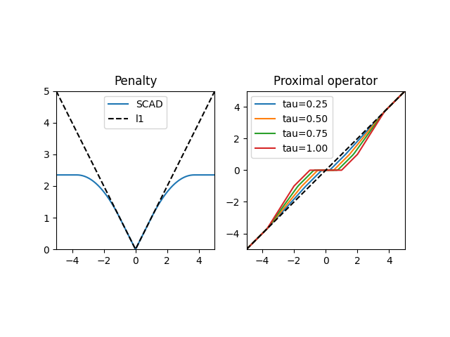
The SCAD penalty combines both soft-thresholding and hard-thresholding in a continuous manner
scad = pyproximal.SCAD(1, 3.7)
compare_penalty_and_proximal_operator(scad)

The Log penalty encourages sparsity more than the l1-penalty and parametrizes a family of functions which lie between l0 and l1-penalties.
log = pyproximal.Log(1, 0.5)
compare_penalty_and_proximal_operator(log)

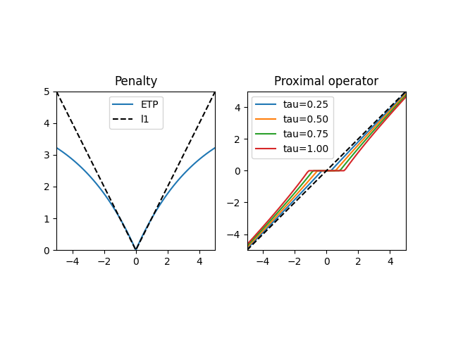
The ETP penalty is similar to the Log penalty in that it tends to the l1-penalty and the l0-penalty at its extremes.
etp = pyproximal.ETP(1, 0.25)
compare_penalty_and_proximal_operator(etp)

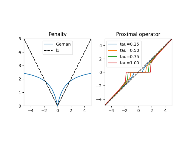
The Geman penalty
geman = pyproximal.Geman(3, 1.2)
compare_penalty_and_proximal_operator(geman)

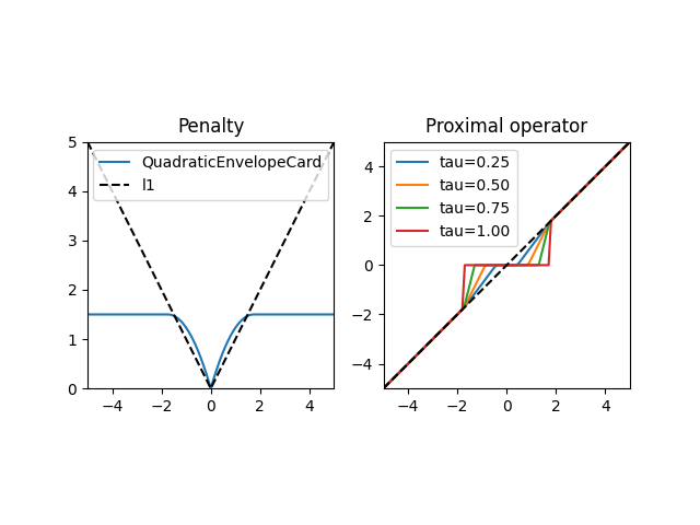
The quadratic envelope of the l0-penalty
f_mu = pyproximal.QuadraticEnvelopeCard(1.5)
compare_penalty_and_proximal_operator(f_mu)

Total running time of the script: (0 minutes 0.908 seconds)
