Note
Go to the end to download the full example code.
Adaptive Primal-Dual#
This tutorial compares the traditional Chambolle-Pock Primal-dual algorithm with the Adaptive Primal-Dual Hybrid Gradient of Goldstein and co-authors.
By adaptively changing the step size in the primal and the dual directions, this algorithm shows faster convergence, which is of great importance for some of the problems that the Primal-Dual algorithm can solve - especially those with an expensive proximal operator.
For this example, we consider a simple denoising problem.
import numpy as np
import matplotlib.pyplot as plt
import pylops
from skimage.data import camera

import pyproximal

plt.close('all')

def callback(x, f, g, K, cost, xtrue, err):
    cost.append(f(x) + g(K.matvec(x)))
    err.append(np.linalg.norm(x - xtrue))
Let’s start by loading a sample image and adding some noise
We can now define a pylops.Gradient operator as well as the
different proximal operators to be passed to our solvers
# Gradient operator
sampling = 1.
Gop = pylops.Gradient(dims=(ny, nx), sampling=sampling, edge=False,
                      kind='forward', dtype='float64')
L = 8. / sampling ** 2 # maxeig(Gop^H Gop)

# L2 data term
lamda = .04
l2 = pyproximal.L2(b=noise_img.ravel(), sigma=lamda)

# L1 regularization (isotropic TV)
l1iso = pyproximal.L21(ndim=2)
To start, we solve our denoising problem with the original Primal-Dual algorithm
# Primal-dual
tau = 0.95 / np.sqrt(L)
mu = 0.95 / np.sqrt(L)

cost_fixed = []
err_fixed = []
iml12_fixed = \
    pyproximal.optimization.primaldual.PrimalDual(l2, l1iso, Gop,
                                                  tau=tau, mu=mu, theta=1.,
                                                  x0=np.zeros_like(img.ravel()),
                                                  gfirst=False, niter=300, show=True,
                                                  callback=lambda x: callback(x, l2, l1iso,
                                                                              Gop, cost_fixed,
                                                                              img.ravel(),
                                                                              err_fixed))
iml12_fixed = iml12_fixed.reshape(img.shape)
Primal-dual: min_x f(Ax) + x^T z + g(x)
---------------------------------------------------------
Proximal operator (f): <class 'pyproximal.proximal.L2.L2'>
Proximal operator (g): <class 'pyproximal.proximal.L21.L21'>
Linear operator (A): <class 'pylops.basicoperators.gradient.Gradient'>
Additional vector (z): None
tau = 0.33587572106361          mu = 0.33587572106361
theta = 1.00            niter = 300

   Itn       x[0]          f           g          z^x       J = f + g + z^x
     1   2.54961e+00   1.147e+08   1.329e+05   0.000e+00       1.148e+08
     2   5.05255e+00   1.117e+08   1.382e+05   0.000e+00       1.119e+08
     3   7.55087e+00   1.089e+08   1.215e+05   0.000e+00       1.090e+08
     4   1.00694e+01   1.061e+08   1.115e+05   0.000e+00       1.062e+08
     5   1.26065e+01   1.034e+08   1.110e+05   0.000e+00       1.035e+08
     6   1.51456e+01   1.007e+08   1.144e+05   0.000e+00       1.008e+08
     7   1.76685e+01   9.813e+07   1.189e+05   0.000e+00       9.825e+07
     8   2.01617e+01   9.562e+07   1.242e+05   0.000e+00       9.574e+07
     9   2.26168e+01   9.317e+07   1.306e+05   0.000e+00       9.330e+07
    10   2.50296e+01   9.078e+07   1.376e+05   0.000e+00       9.092e+07
    31   6.77163e+01   5.295e+07   2.883e+05   0.000e+00       5.324e+07
    61   1.11288e+02   2.517e+07   4.542e+05   0.000e+00       2.563e+07
    91   1.40757e+02   1.266e+07   5.673e+05   0.000e+00       1.323e+07
   121   1.60379e+02   7.016e+06   6.433e+05   0.000e+00       7.659e+06
   151   1.73596e+02   4.465e+06   6.942e+05   0.000e+00       5.160e+06
   181   1.82419e+02   3.309e+06   7.284e+05   0.000e+00       4.037e+06
   211   1.88331e+02   2.782e+06   7.513e+05   0.000e+00       3.533e+06
   241   1.92292e+02   2.540e+06   7.666e+05   0.000e+00       3.307e+06
   271   1.94945e+02   2.428e+06   7.769e+05   0.000e+00       3.205e+06
   292   1.96263e+02   2.388e+06   7.820e+05   0.000e+00       3.170e+06
   293   1.96317e+02   2.386e+06   7.822e+05   0.000e+00       3.169e+06
   294   1.96371e+02   2.385e+06   7.824e+05   0.000e+00       3.167e+06
   295   1.96423e+02   2.384e+06   7.826e+05   0.000e+00       3.166e+06
   296   1.96475e+02   2.382e+06   7.828e+05   0.000e+00       3.165e+06
   297   1.96526e+02   2.381e+06   7.830e+05   0.000e+00       3.164e+06
   298   1.96577e+02   2.380e+06   7.832e+05   0.000e+00       3.163e+06
   299   1.96627e+02   2.378e+06   7.834e+05   0.000e+00       3.162e+06
   300   1.96676e+02   2.377e+06   7.836e+05   0.000e+00       3.161e+06

Total time (s) = 5.19
---------------------------------------------------------
We do the same with the adaptive algorithm
cost_ada = []
err_ada = []
iml12_ada, steps = \
    pyproximal.optimization.primaldual.AdaptivePrimalDual(l2, l1iso, Gop,
                                                          tau=tau, mu=mu,
                                                          x0=np.zeros_like(img.ravel()),
                                                          niter=45, show=True, tol=0.05,
                                                          callback=lambda x: callback(x, l2, l1iso,
                                                                                      Gop, cost_ada,
                                                                                      img.ravel(),
                                                                                      err_ada))
iml12_ada = iml12_ada.reshape(img.shape)
Adaptive Primal-dual: min_x f(Ax) + x^T z + g(x)
---------------------------------------------------------
Proximal operator (f): <class 'pyproximal.proximal.L2.L2'>
Proximal operator (g): <class 'pyproximal.proximal.L21.L21'>
Linear operator (A): <class 'pylops.basicoperators.gradient.Gradient'>
Additional vector (z): None
tau0 = 3.358757e-01     mu0 = 3.358757e-01
alpha0 = 5.000000e-01   eta = 9.500000e-01
s = 1.000000e+00        delta = 1.500000e+00
niter = 45              tol = 5.000000e-02

   Itn       x[0]          f           g          z^x       J = f + g + z^x
     2   2.54961e+00   1.147e+08   1.329e+05   0.000e+00       1.148e+08
     3   7.48999e+00   1.089e+08   1.622e+05   0.000e+00       1.090e+08
     4   1.65571e+01   9.877e+07   2.028e+05   0.000e+00       9.898e+07
     5   3.19051e+01   8.306e+07   2.861e+05   0.000e+00       8.335e+07
     6   5.52202e+01   6.205e+07   4.082e+05   0.000e+00       6.246e+07
     7   8.62168e+01   3.911e+07   5.574e+05   0.000e+00       3.966e+07
     8   1.10593e+02   2.498e+07   6.663e+05   0.000e+00       2.565e+07
     9   1.29773e+02   1.629e+07   7.415e+05   0.000e+00       1.703e+07
    10   1.44869e+02   1.093e+07   7.926e+05   0.000e+00       1.172e+07
    13   1.71060e+02   4.725e+06   8.581e+05   0.000e+00       5.583e+06
    17   1.77932e+02   3.754e+06   8.468e+05   0.000e+00       4.601e+06
    21   1.82074e+02   3.304e+06   8.338e+05   0.000e+00       4.137e+06
    25   1.86241e+02   2.929e+06   8.436e+05   0.000e+00       3.772e+06
    29   1.89192e+02   2.694e+06   8.347e+05   0.000e+00       3.528e+06
    33   1.91291e+02   2.554e+06   8.174e+05   0.000e+00       3.371e+06
    37   1.93240e+02   2.468e+06   8.066e+05   0.000e+00       3.275e+06
    38   1.93720e+02   2.452e+06   8.050e+05   0.000e+00       3.257e+06
    39   1.94188e+02   2.438e+06   8.037e+05   0.000e+00       3.242e+06
    40   1.94640e+02   2.426e+06   8.027e+05   0.000e+00       3.228e+06
    41   1.95070e+02   2.415e+06   8.018e+05   0.000e+00       3.216e+06
    42   1.95472e+02   2.405e+06   8.012e+05   0.000e+00       3.206e+06
    43   1.95843e+02   2.396e+06   8.007e+05   0.000e+00       3.197e+06
    44   1.96181e+02   2.389e+06   8.003e+05   0.000e+00       3.189e+06
    45   1.96484e+02   2.382e+06   8.000e+05   0.000e+00       3.182e+06
    46   1.96752e+02   2.376e+06   7.998e+05   0.000e+00       3.176e+06

Total time (s) = 0.88
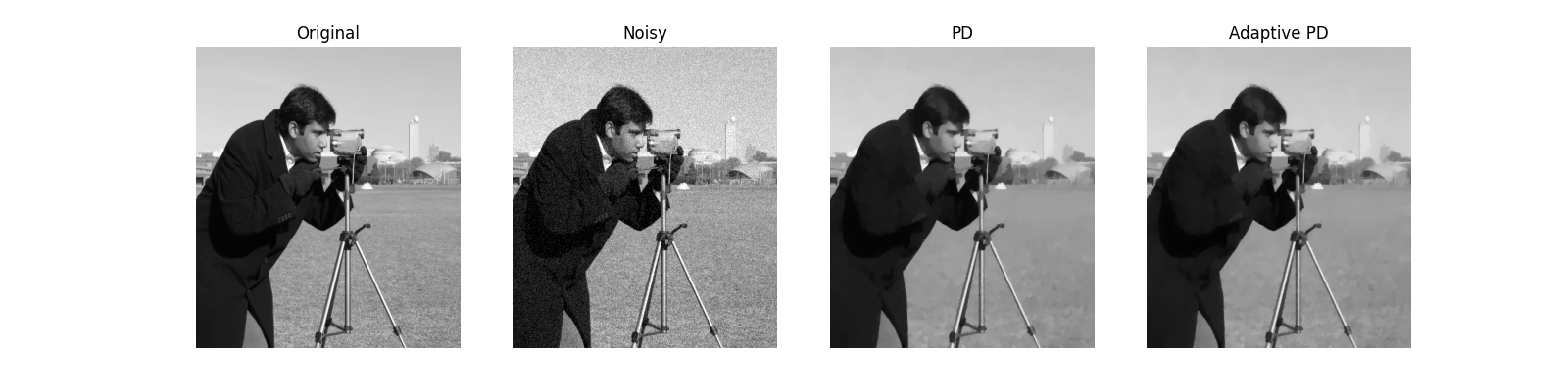
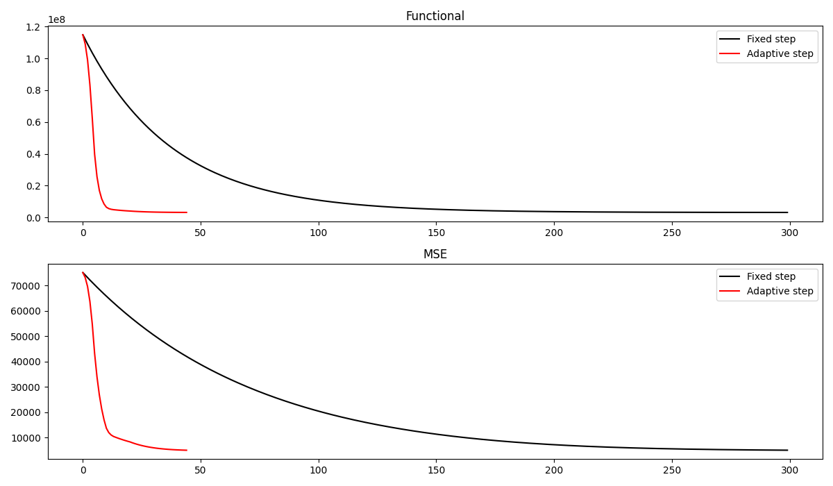
Let’s now compare the final results as well as the convergence curves of the two algorithms. We can see how the adaptive Primal-Dual produces a better estimate of the clean image in a much smaller number of iterations
fig, axs = plt.subplots(1, 4, figsize=(16, 4))
axs[0].imshow(img, cmap='gray', vmin=0, vmax=255)
axs[0].set_title('Original')
axs[0].axis('off')
axs[0].axis('tight')
axs[1].imshow(noise_img, cmap='gray', vmin=0, vmax=255)
axs[1].set_title('Noisy')
axs[1].axis('off')
axs[1].axis('tight')
axs[2].imshow(iml12_fixed, cmap='gray', vmin=0, vmax=255)
axs[2].set_title('PD')
axs[2].axis('off')
axs[2].axis('tight')
axs[3].imshow(iml12_ada, cmap='gray', vmin=0, vmax=255)
axs[3].set_title('Adaptive PD')
axs[3].axis('off')
axs[3].axis('tight')
fig, axs = plt.subplots(2, 1, figsize=(12, 7))
axs[0].plot(cost_fixed, 'k', label='Fixed step')
axs[0].plot(cost_ada, 'r', label='Adaptive step')
axs[0].legend()
axs[0].set_title('Functional')
axs[1].plot(err_fixed, 'k', label='Fixed step')
axs[1].plot(err_ada, 'r', label='Adaptive step')
axs[1].set_title('MSE')
axs[1].legend()
plt.tight_layout()
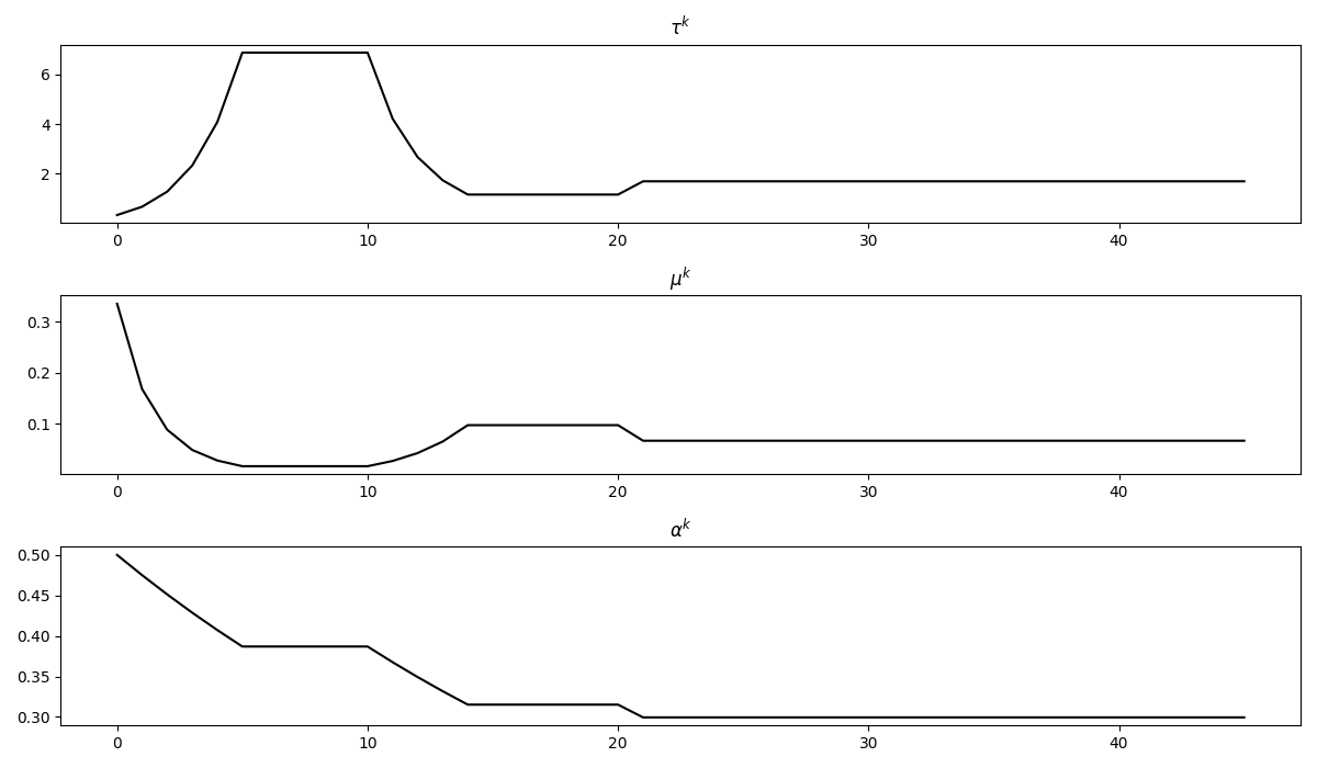
fig, axs = plt.subplots(3, 1, figsize=(12, 7))
axs[0].plot(steps[0], 'k')
axs[0].set_title(r'$\tau^k$')
axs[1].plot(steps[1], 'k')
axs[1].set_title(r'$\mu^k$')
axs[2].plot(steps[2], 'k')
axs[2].set_title(r'$\alpha^k$')
plt.tight_layout();
Total running time of the script: (0 minutes 6.597 seconds)