
Note
Go to the end to download the full example code.
Adaptive Primal-Dual#
This tutorial compares the traditional Chambolle-Pock Primal-dual algorithm with the Adaptive Primal-Dual Hybrid Gradient of Goldstein and co-authors.
By adaptively changing the step size in the primal and the dual directions, this algorithm shows faster convergence, which is of great importance for some of the problems that the Primal-Dual algorithm can solve - especially those with an expensive proximal operator.
For this example, we consider a simple denoising problem.
import numpy as np
import matplotlib.pyplot as plt
import pylops
from skimage.data import camera

import pyproximal

plt.close('all')

def callback(x, f, g, K, cost, xtrue, err):
    cost.append(f(x) + g(K.matvec(x)))
    err.append(np.linalg.norm(x - xtrue))
Let’s start by loading a sample image and adding some noise
We can now define a pylops.Gradient operator as well as the
different proximal operators to be passed to our solvers
# Gradient operator
sampling = 1.
Gop = pylops.Gradient(dims=(ny, nx), sampling=sampling, edge=False,
                      kind='forward', dtype='float64')
L = 8. / sampling ** 2 # maxeig(Gop^H Gop)

# L2 data term
lamda = .04
l2 = pyproximal.L2(b=noise_img.ravel(), sigma=lamda)

# L1 regularization (isotropic TV)
l1iso = pyproximal.L21(ndim=2)
To start, we solve our denoising problem with the original Primal-Dual algorithm
# Primal-dual
tau = 0.95 / np.sqrt(L)
mu = 0.95 / np.sqrt(L)

cost_fixed = []
err_fixed = []
iml12_fixed = \
    pyproximal.optimization.primaldual.PrimalDual(l2, l1iso, Gop,
                                                  tau=tau, mu=mu, theta=1.,
                                                  x0=np.zeros_like(img.ravel()),
                                                  gfirst=False, niter=300, show=True,
                                                  callback=lambda x: callback(x, l2, l1iso,
                                                                              Gop, cost_fixed,
                                                                              img.ravel(),
                                                                              err_fixed))
iml12_fixed = iml12_fixed.reshape(img.shape)
Primal-dual: min_x f(Ax) + x^T z + g(x)
---------------------------------------------------------
Proximal operator (f): <class 'pyproximal.proximal.L2.L2'>
Proximal operator (g): <class 'pyproximal.proximal.L21.L21'>
Linear operator (A): <class 'pylops.basicoperators.gradient.Gradient'>
Additional vector (z): None
tau = 0.33587572106361          mu = 0.33587572106361
theta = 1.00            niter = 300

   Itn       x[0]          f           g          z^x       J = f + g + z^x
     1   2.55225e+00   1.147e+08   1.331e+05   0.000e+00       1.149e+08
     2   4.95447e+00   1.118e+08   1.384e+05   0.000e+00       1.119e+08
     3   7.32107e+00   1.089e+08   1.216e+05   0.000e+00       1.090e+08
     4   9.70895e+00   1.061e+08   1.114e+05   0.000e+00       1.062e+08
     5   1.21188e+01   1.034e+08   1.107e+05   0.000e+00       1.035e+08
     6   1.45291e+01   1.008e+08   1.141e+05   0.000e+00       1.009e+08
     7   1.69219e+01   9.819e+07   1.186e+05   0.000e+00       9.830e+07
     8   1.92914e+01   9.567e+07   1.239e+05   0.000e+00       9.580e+07
     9   2.16414e+01   9.322e+07   1.303e+05   0.000e+00       9.335e+07
    10   2.39798e+01   9.084e+07   1.373e+05   0.000e+00       9.097e+07
    31   6.70599e+01   5.298e+07   2.885e+05   0.000e+00       5.327e+07
    61   1.10590e+02   2.519e+07   4.549e+05   0.000e+00       2.564e+07
    91   1.39931e+02   1.267e+07   5.685e+05   0.000e+00       1.323e+07
   121   1.59453e+02   7.019e+06   6.447e+05   0.000e+00       7.663e+06
   151   1.72525e+02   4.466e+06   6.957e+05   0.000e+00       5.162e+06
   181   1.81239e+02   3.309e+06   7.300e+05   0.000e+00       4.039e+06
   211   1.87092e+02   2.782e+06   7.529e+05   0.000e+00       3.535e+06
   241   1.91023e+02   2.540e+06   7.683e+05   0.000e+00       3.308e+06
   271   1.93648e+02   2.428e+06   7.786e+05   0.000e+00       3.207e+06
   292   1.94953e+02   2.387e+06   7.838e+05   0.000e+00       3.171e+06
   293   1.95007e+02   2.386e+06   7.840e+05   0.000e+00       3.170e+06
   294   1.95060e+02   2.384e+06   7.842e+05   0.000e+00       3.169e+06
   295   1.95113e+02   2.383e+06   7.844e+05   0.000e+00       3.167e+06
   296   1.95166e+02   2.382e+06   7.846e+05   0.000e+00       3.166e+06
   297   1.95217e+02   2.380e+06   7.848e+05   0.000e+00       3.165e+06
   298   1.95268e+02   2.379e+06   7.850e+05   0.000e+00       3.164e+06
   299   1.95318e+02   2.378e+06   7.852e+05   0.000e+00       3.163e+06
   300   1.95368e+02   2.377e+06   7.854e+05   0.000e+00       3.162e+06

Total time (s) = 6.65
---------------------------------------------------------
We do the same with the adaptive algorithm
cost_ada = []
err_ada = []
iml12_ada, steps = \
    pyproximal.optimization.primaldual.AdaptivePrimalDual(l2, l1iso, Gop,
                                                          tau=tau, mu=mu,
                                                          x0=np.zeros_like(img.ravel()),
                                                          niter=45, show=True, tol=0.05,
                                                          callback=lambda x: callback(x, l2, l1iso,
                                                                                      Gop, cost_ada,
                                                                                      img.ravel(),
                                                                                      err_ada))
iml12_ada = iml12_ada.reshape(img.shape)
Adaptive Primal-dual: min_x f(Ax) + x^T z + g(x)
---------------------------------------------------------
Proximal operator (f): <class 'pyproximal.proximal.L2.L2'>
Proximal operator (g): <class 'pyproximal.proximal.L21.L21'>
Linear operator (A): <class 'pylops.basicoperators.gradient.Gradient'>
Additional vector (z): None
tau0 = 3.358757e-01     mu0 = 3.358757e-01
alpha0 = 5.000000e-01   eta = 9.500000e-01
s = 1.000000e+00        delta = 1.500000e+00
niter = 45              tol = 5.000000e-02

   Itn       x[0]          f           g          z^x       J = f + g + z^x
     2   2.55225e+00   1.147e+08   1.331e+05   0.000e+00       1.149e+08
     3   7.29382e+00   1.089e+08   1.624e+05   0.000e+00       1.091e+08
     4   1.59759e+01   9.883e+07   2.027e+05   0.000e+00       9.903e+07
     5   3.06967e+01   8.311e+07   2.854e+05   0.000e+00       8.340e+07
     6   5.30254e+01   6.209e+07   4.068e+05   0.000e+00       6.250e+07
     7   8.26519e+01   3.913e+07   5.551e+05   0.000e+00       3.969e+07
     8   1.05944e+02   2.500e+07   6.635e+05   0.000e+00       2.566e+07
     9   1.24300e+02   1.630e+07   7.386e+05   0.000e+00       1.704e+07
    10   1.38814e+02   1.094e+07   7.896e+05   0.000e+00       1.173e+07
    13   1.64419e+02   4.730e+06   8.553e+05   0.000e+00       5.585e+06
    17   1.71883e+02   3.758e+06   8.445e+05   0.000e+00       4.602e+06
    21   1.77391e+02   3.307e+06   8.321e+05   0.000e+00       4.139e+06
    25   1.82697e+02   2.931e+06   8.428e+05   0.000e+00       3.774e+06
    29   1.87108e+02   2.695e+06   8.346e+05   0.000e+00       3.530e+06
    33   1.89833e+02   2.555e+06   8.179e+05   0.000e+00       3.372e+06
    37   1.91793e+02   2.468e+06   8.076e+05   0.000e+00       3.276e+06
    38   1.92212e+02   2.452e+06   8.061e+05   0.000e+00       3.258e+06
    39   1.92599e+02   2.438e+06   8.048e+05   0.000e+00       3.243e+06
    40   1.92953e+02   2.426e+06   8.039e+05   0.000e+00       3.230e+06
    41   1.93278e+02   2.415e+06   8.031e+05   0.000e+00       3.218e+06
    42   1.93577e+02   2.405e+06   8.026e+05   0.000e+00       3.208e+06
    43   1.93857e+02   2.396e+06   8.022e+05   0.000e+00       3.198e+06
    44   1.94120e+02   2.389e+06   8.019e+05   0.000e+00       3.190e+06
    45   1.94371e+02   2.382e+06   8.016e+05   0.000e+00       3.183e+06
    46   1.94611e+02   2.376e+06   8.014e+05   0.000e+00       3.177e+06

Total time (s) = 1.19
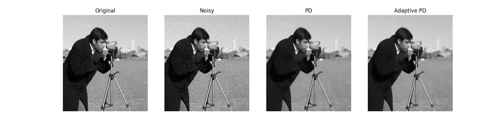
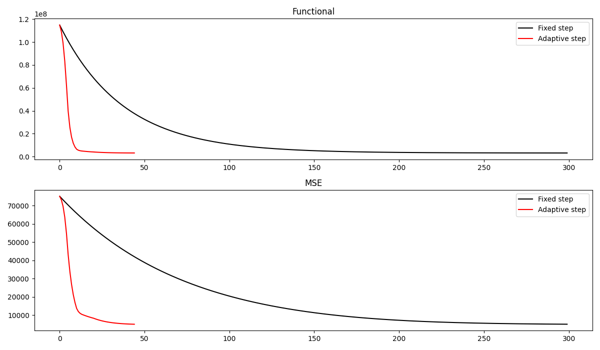
Let’s now compare the final results as well as the convergence curves of the two algorithms. We can see how the adaptive Primal-Dual produces a better estimate of the clean image in a much smaller number of iterations
fig, axs = plt.subplots(1, 4, figsize=(16, 4))
axs[0].imshow(img, cmap='gray', vmin=0, vmax=255)
axs[0].set_title('Original')
axs[0].axis('off')
axs[0].axis('tight')
axs[1].imshow(noise_img, cmap='gray', vmin=0, vmax=255)
axs[1].set_title('Noisy')
axs[1].axis('off')
axs[1].axis('tight')
axs[2].imshow(iml12_fixed, cmap='gray', vmin=0, vmax=255)
axs[2].set_title('PD')
axs[2].axis('off')
axs[2].axis('tight')
axs[3].imshow(iml12_ada, cmap='gray', vmin=0, vmax=255)
axs[3].set_title('Adaptive PD')
axs[3].axis('off')
axs[3].axis('tight')
fig, axs = plt.subplots(2, 1, figsize=(12, 7))
axs[0].plot(cost_fixed, 'k', label='Fixed step')
axs[0].plot(cost_ada, 'r', label='Adaptive step')
axs[0].legend()
axs[0].set_title('Functional')
axs[1].plot(err_fixed, 'k', label='Fixed step')
axs[1].plot(err_ada, 'r', label='Adaptive step')
axs[1].set_title('MSE')
axs[1].legend()
plt.tight_layout()
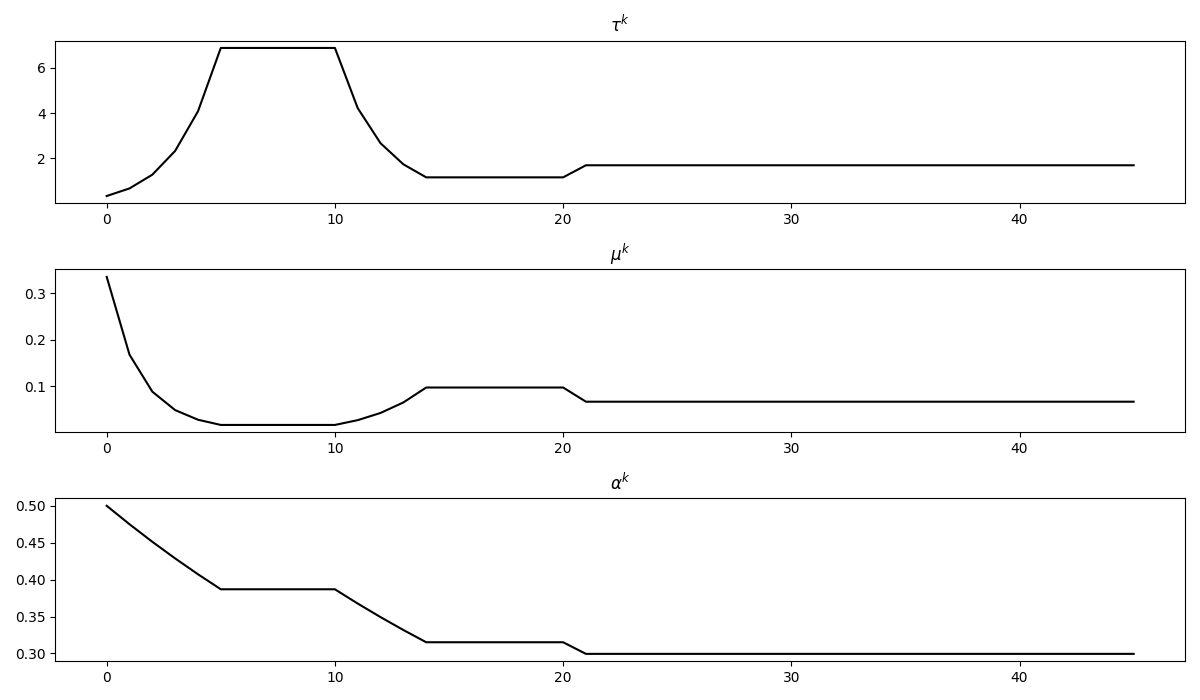
fig, axs = plt.subplots(3, 1, figsize=(12, 7))
axs[0].plot(steps[0], 'k')
axs[0].set_title(r'$\tau^k$')
axs[1].plot(steps[1], 'k')
axs[1].set_title(r'$\mu^k$')
axs[2].plot(steps[2], 'k')
axs[2].set_title(r'$\alpha^k$')
plt.tight_layout();
Total running time of the script: (0 minutes 8.666 seconds)