pyproximal.L2
- class pyproximal.L2(Op: LinearOperator | None = None, b: ndarray[tuple[Any, ...], dtype[_ScalarT]] | None = None, q: ndarray[tuple[Any, ...], dtype[_ScalarT]] | None = None, sigma: float = 1.0, alpha: float = 1.0, qgrad: bool = True, niter: int | Callable[[int], int] = 10, x0: ndarray[tuple[Any, ...], dtype[_ScalarT]] | None = None, warm: bool = True, solver: str | None = 'legacy', densesolver: str | None = None, kwargs_solver: dict[str, Any] | None = None)[source]
L2 Norm proximal operator.
The Proximal operator of the \(\ell_2\) norm is defined as: \(f(\mathbf{x}) = \frac{\sigma}{2} ||\mathbf{Op}\mathbf{x} - \mathbf{b}||_2^2\) and \(f_\alpha(\mathbf{x}) = f(\mathbf{x}) + \alpha \mathbf{q}^T\mathbf{x}\).
- Parameters:
- Op
pylops.LinearOperator, optional Linear operator
- b
numpy.ndarray, optional Data vector
- q
numpy.ndarray, optional Dot vector
- sigma
int, optional Multiplicative coefficient of L2 norm
- alpha
float, optional Multiplicative coefficient of dot product
- qgrad
bool, optional Add q term to gradient (
True) or not (False)- niter
intorfunc, optional Number of iterations of iterative scheme used to compute the proximal. This can be a constant number or a function that is called passing a counter which keeps track of how many times the
proxmethod has been invoked before and returns theniterto be used.- x0
numpy.ndarray, optional Initial vector
- warm
bool, optional Warm start (
True) or not (False). Uses estimate from previous call ofproxmethod.- solver
str, optional Added in version 0.11.0.
Name of solver to use with non-explicit operators:
legacy: enforces the legacy behaviour wherescipy.sparse.linalg.lsqris used with numpy data andpylops.optimization.basic.lsqris used with cupy data (both are applied to the normal equations);cgto usepylops.optimization.basic.cgon the normal equations;cglsto usepylops.optimization.basic.cglson the regularized system of equations;
- densesolver
str, optional Use
numpy,scipy, orfactorizewhen dealing with explicit operators. The former two rely on dense solvers from either library, whilst the last computes a factorization of the matrix to invert and avoids to do so unless the \(\tau\) or \(\sigma\) paramets have changed. Choosedensesolver=Nonewhen using PyLops versions earlier than v1.18.1 or v2.0.0- **kwargs_solver
dict, optional Dictionary containing extra arguments for the solver selected via the
solverparameter.
- Op
Notes
The L2 proximal operator is defined as:
\[prox_{\tau f_\alpha}(\mathbf{x}) = \left(\mathbf{I} + \tau \sigma \mathbf{Op}^T \mathbf{Op} \right)^{-1} \left( \mathbf{x} + \tau \sigma \mathbf{Op}^T \mathbf{b} - \tau \alpha \mathbf{q}\right)\]when both
Opandbare provided. This formula shows that the proximal operator requires the solution of an inverse problem. If the operatorOpis of kindexplicit=True, we can solve this problem directly. On the other hand ifOpis of kindexplicit=False, an iterative solver is employed. In this case it is possible to provide a warm start via thex0input parameter.Note that alternatively the proximal operator can be computed solving the following augumented system of equations (instead of its normal equations as shown above):
\[\begin{split}\begin{bmatrix} \sqrt{\tau \sigma} \mathbf{Op} \\ \mathbf{I} \end{bmatrix} prox_{\tau f_\alpha}(\mathbf{x}) = \begin{bmatrix} \sqrt{\tau \sigma} \mathbf{b} \\ \mathbf{x} - \tau \alpha \mathbf{q} \end{bmatrix}\end{split}\]The choice of the parameter
solverdetermines which of the two approaches is used.Alternatively, when only
bis provided,Opis assumed to be an Identity operator and the proximal operator reduces to:\[\prox_{\tau f_\alpha}(\mathbf{x}) = \frac{\mathbf{x} + \tau \sigma \mathbf{b} - \tau \alpha \mathbf{q}} {1 + \tau \sigma}\]If
bis not provided, the proximal operator reduces to:\[\prox_{\tau f_\alpha}(\mathbf{x}) = \frac{\mathbf{x} - \tau \alpha \mathbf{q}}{1 + \tau \sigma}\]Finally, note that the second term in \(f_\alpha(\mathbf{x})\) is added because this combined expression appears in several problems where Bregman iterations are used alongside a proximal solver.
Methods
__init__([Op, b, q, sigma, alpha, qgrad, ...])affine_addition(v)Affine addition
chain(g)Chain
grad(x)Gradient of the Moreau envelope of the function.
postcomposition(sigma)Postcomposition
precomposition(a, b)Precomposition
prox(*args, **kwargs)proxdual(**kwargs)
Examples using pyproximal.L2
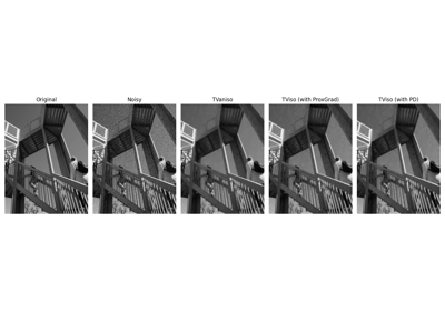
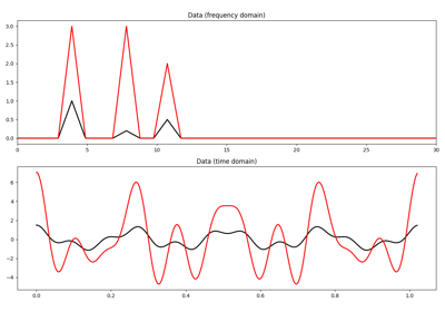
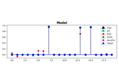
IHT, ISTA, FISTA, AA-ISTA, and TWIST for Compressive sensing