Norms

This example shows how to compute proximal operators of different norms, namely:

• Euclidean norm (pyproximal.Euclidean)

• L2 norm (pyproximal.L2)

• L1 norm (pyproximal.L1)

• L21 norm (pyproximal.L21)

import matplotlib.pyplot as plt
import numpy as np
import pylops

import pyproximal

plt.close("all")

Let’s start with the Euclidean norm. We define a vector \(\mathbf{x}\) and a scalar \(\sigma\) and compute the norm. We then define the proximal scalar \(\tau\) and compute the proximal operator and its dual.

eucl = pyproximal.Euclidean(sigma=2.0)

x = np.arange(-1, 1, 0.1)
print("||x||_2: ", eucl(x))

tau = 2
xp = eucl.prox(x, tau)
xdp = eucl.proxdual(x, tau)

plt.figure(figsize=(7, 2))
plt.plot(x, x, "k", lw=2, label="x")
plt.plot(x, xp, "r", lw=2, label="prox(x)")
plt.plot(x, xdp, "b", lw=2, label="dualprox(x)")
plt.xlabel("x")
plt.title(r"$||x||_2$")
plt.legend()
plt.tight_layout()

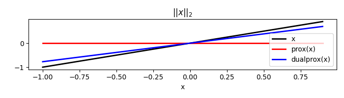
||x||_2:  5.176871642217913

Similarly we can do the same for the L2 norm (i.e., square of Euclidean norm)

l2 = pyproximal.L2(sigma=2.0)

x = np.arange(-1, 1, 0.1)
print("||x||_2^2: ", l2(x))

tau = 2
xp = l2.prox(x, tau)
xdp = l2.proxdual(x, tau)

plt.figure(figsize=(7, 2))
plt.plot(x, x, "k", lw=2, label="x")
plt.plot(x, xp, "r", lw=2, label="prox(x)")
plt.plot(x, xdp, "b", lw=2, label="dualprox(x)")
plt.xlabel("x")
plt.title(r"$||x||_2^2$")
plt.legend()
plt.tight_layout()

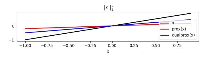
||x||_2^2:  6.6999999999999975

For this norm we can also subtract a vector to x and multiply x by a matrix A

l2 = pyproximal.L2(sigma=2.0, b=np.ones_like(x))

x = np.arange(-1, 1, 0.1)
print("||x-b||_2^2: ", l2(x))

tau = 2
xp = l2.prox(x, tau)
xdp = l2.proxdual(x, tau)

plt.figure(figsize=(7, 2))
plt.plot(x, x, "k", lw=2, label="x")
plt.plot(x, xp, "r", lw=2, label="prox(x)")
plt.plot(x, xdp, "b", lw=2, label="dualprox(x)")
plt.xlabel("x")
plt.title(r"$||x-b||_2^2$")
plt.legend()
plt.tight_layout()

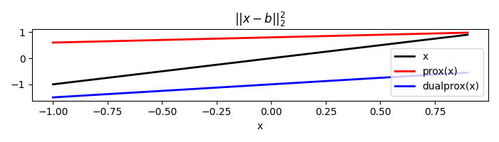
||x-b||_2^2:  28.70000000000001

Finally we can also multiply x by a matrix A

x = np.arange(-1, 1, 0.1)
nx = len(x)
ny = nx * 2
A = np.random.normal(0, 1, (ny, nx))

l2 = pyproximal.L2(sigma=2.0, b=np.ones(ny), Op=pylops.MatrixMult(A))
print("||Ax-b||_2^2: ", l2(x))

tau = 2
xp = l2.prox(x, tau)
xdp = l2.proxdual(x, tau)

plt.figure(figsize=(7, 2))
plt.plot(x, x, "k", lw=2, label="x")
plt.plot(x, xp, "r", lw=2, label="prox(x)")
plt.plot(x, xdp, "b", lw=2, label="dualprox(x)")
plt.xlabel("x")
plt.title(r"$||Ax-b||_2^2$")
plt.legend()
plt.tight_layout()

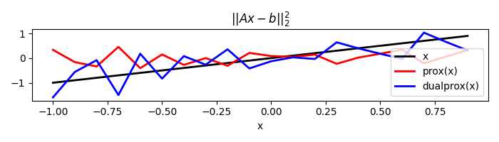
||Ax-b||_2^2:  271.4446529660882

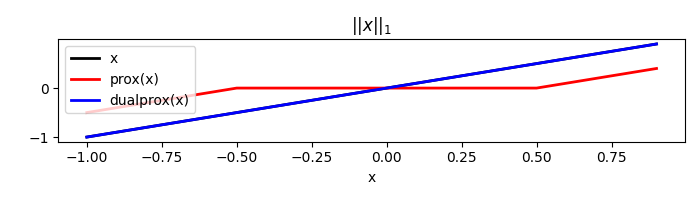
We consider now the L1 norm. Here the proximal operator can be easily computed using the so-called soft-thresholding operation on each element of the input vector

l1 = pyproximal.L1(sigma=1.0)

x = np.arange(-1, 1, 0.1)
print("||x||_1: ", l1(x))

tau = 0.5
xp = l1.prox(x, tau)
xdp = l1.proxdual(x, tau)

plt.figure(figsize=(7, 2))
plt.plot(x, x, "k", lw=2, label="x")
plt.plot(x, xp, "r", lw=2, label="prox(x)")
plt.plot(x, xdp, "b", lw=2, label="dualprox(x)")
plt.xlabel("x")
plt.title(r"$||x||_1$")
plt.legend()
plt.tight_layout()

||x||_1:  9.999999999999996

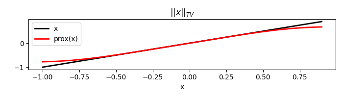
We consider now the TV norm.

tv = pyproximal.TV(dims=(nx,), sigma=1.0)

x = np.arange(-1, 1, 0.1)
print("||x||_{TV}: ", l1(x))

tau = 0.5
xp = tv.prox(x, tau)

plt.figure(figsize=(7, 2))
plt.plot(x, x, "k", lw=2, label="x")
plt.plot(x, xp, "r", lw=2, label="prox(x)")
plt.xlabel("x")
plt.title(r"$||x||_{TV}$")
plt.legend()
plt.tight_layout()

||x||_{TV}:  9.999999999999996

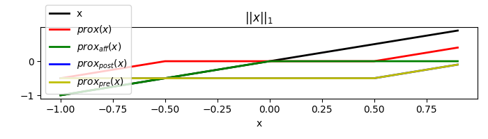
Finally, moving back to the L1 norm, let’s consider a number of basic operation that still lead to known and easy to compute proximal operator, namely:

• affine addition: add the product of a vector \(\mathbf{v}\) with \(\mathbf{x}\) (i.e., \(+ \mathbf{v}^H \mathbf{x}\)) - accessed via the + operator

• post-composition: multiply the L1 norm with a scalar \(\sigma\)

• pre-composition: multiply \(\mathbf{x}\) with a scalar \(a\) and sum with a scalar or vector \(\mathbf{b}\)

x = np.arange(-1, 1, 0.1)

l1 = pyproximal.L1(sigma=1.0)

l1_affine = l1 + np.ones_like(x)
l1_postcomp = l1.postcomposition(2.0)
l1_precomp = l1.precomposition(2.0, np.ones_like(x))

print("||x||_1: ", l1(x))
print("||x||_1 + v^T x: ", l1_affine(x))
print("σ ||x||_1: ", l1_postcomp(x))
print("||a x + b||_1: ", l1_precomp(x))

l1_affine = l1 + np.ones_like(x)
l1_postcomp = l1.postcomposition(2.0)
l1_precomp = l1.precomposition(2.0, np.ones_like(x))

tau = 0.5
xp = l1.prox(x, tau)
xp_affine = l1_affine.prox(x, tau)
xp_postcomp = l1_postcomp.prox(x, tau)
xp_precomp = l1_precomp.prox(x, tau)

plt.figure(figsize=(7, 2))
plt.plot(x, x, "k", lw=2, label="x")
plt.plot(x, xp, "r", lw=2, label=r"$prox(x)$")
plt.plot(x, xp_affine, "g", lw=2, label=r"$prox_{aff}(x)$")
plt.plot(x, xp_precomp, "b", lw=2, label=r"$prox_{post}(x)$")
plt.plot(x, xp_precomp, "y", lw=2, label=r"$prox_{pre}(x)$")
plt.xlabel("x")
plt.title(r"$||x||_1$")
plt.legend()
plt.tight_layout()

||x||_1:  9.999999999999996
||x||_1 + v^T x:  8.999999999999993
σ ||x||_1:  19.999999999999993
||a x + b||_1:  23.999999999999993