Note
Go to the end to download the full example code.
Deblending
This is the continuation of the deblending tutorial in PyLops, where a novel approach
to deblending using a hard-data constraint is implementent [1].
In other words, we aim to solve the following problem:
where \(\mathbf{d} = [\mathbf{d}_1^T, \mathbf{d}_2^T,\ldots,
\mathbf{d}_N^T]^T\) is a stack of \(N\) individual shot gathers,
\(\boldsymbol\Phi=[\boldsymbol\Phi_1, \boldsymbol\Phi_2,\ldots,
\boldsymbol\Phi_N]\) is the blending operator, \(\mathbf{d}^b\) is the
so-called supergather than contains all shots superimposed to each other,
\(\mathbf{S}\) is a patch-FK transform, and \(i_{\mathbf{d}^b-\boldsymbol\Phi \mathbf{d}}\)
is the indicator function of the pyproximal.AffineSet.
import matplotlib.pyplot as plt
import numpy as np
import pylops

import pyproximal

np.random.seed(10)
plt.close("all")
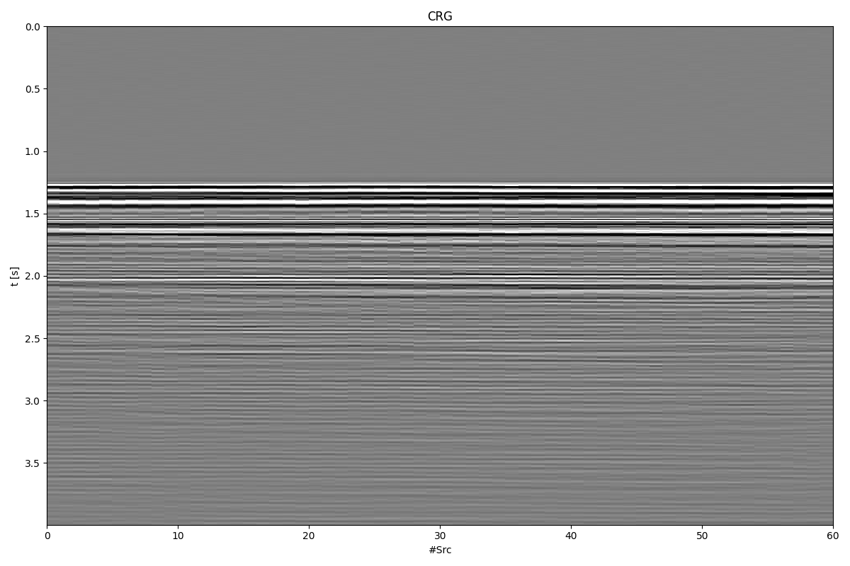
Let’s load and display a small portion of the MobilAVO dataset composed of 60 shots and a single receiver. This data is unblended.
data = np.load("../testdata/mobil.npy")
ns, nt = data.shape

dt = 0.004
t = np.arange(nt) * dt

fig, ax = plt.subplots(1, 1, figsize=(12, 8))
ax.imshow(
    data.T,
    cmap="gray",
    vmin=-50,
    vmax=50,
    extent=(0, ns, t[-1], 0),
    interpolation="none",
)
ax.set_title("CRG")
ax.set_xlabel("#Src")
ax.set_ylabel("t [s]")
ax.axis("tight")
plt.tight_layout()
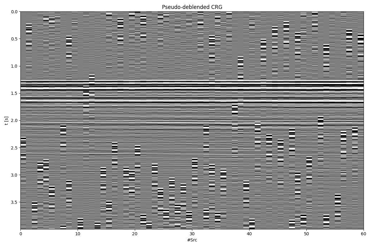
We are now ready to define the blending operator, blend our data, and apply the adjoint of the blending operator to it. This is usually referred as pseudo-deblending: as we will see brings back each source to its own nominal firing time, but since sources partially overlap in time, it will also generate some burst like noise in the data. Deblending can hopefully fix this.
overlap = 0.5
ignition_times = 2.0 * np.random.rand(ns) - 1.0
ignition_times = np.arange(0, overlap * nt * ns, overlap * nt) * dt + ignition_times
ignition_times[0] = 0.0
Bop = pylops.waveeqprocessing.BlendingContinuous(
    nt, 1, ns, dt, ignition_times, dtype="complex128"
)

data_blended = Bop * data[:, np.newaxis]
data_pseudo = Bop.H * data_blended
data_pseudo = data_pseudo.reshape(ns, nt)

fig, ax = plt.subplots(1, 1, figsize=(12, 8))
ax.imshow(
    data_pseudo.T.real,
    cmap="gray",
    vmin=-50,
    vmax=50,
    extent=(0, ns, t[-1], 0),
    interpolation="none",
)
ax.set_title("Pseudo-deblended CRG")
ax.set_xlabel("#Src")
ax.set_ylabel("t [s]")
ax.axis("tight")
plt.tight_layout()
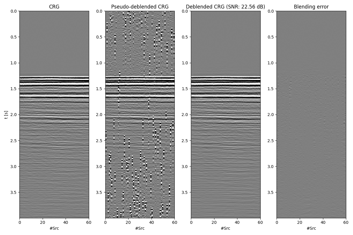
We are finally ready to solve our deblending inverse problem
# Patched FK
dimsd = data.shape
nwin = (20, 80)
nover = (10, 40)
nop = (128, 128)
nop1 = (128, 65)
nwins = (5, 24)
dims = (nwins[0] * nop1[0], nwins[1] * nop1[1])

Fop = pylops.signalprocessing.FFT2D(nwin, nffts=nop, real=True)
Sop = pylops.signalprocessing.Patch2D(
    Fop.H, dims, dimsd, nwin, nover, nop1, tapertype="cosinesqrt"
)
S1op = pylops.signalprocessing.Patch2D(
    Fop.H, dims, dimsd, nwin, nover, nop1, tapertype=None
)

# Define max eigenvalue (we hard-code it here for simplicity)
maxeig = 3

# Define max value in the patch-FK domain for normalization
# and iteration-dependent thresholding
data_fkpatches = (S1op.H @ data_pseudo.ravel()).reshape(Sop.dims)
max_fkpatches = np.abs(data_fkpatches).max()


def sigma(iiter):
    return (max_fkpatches * 0.6) * (0.9**iiter)


# Deblend
niter = 60

tau = 0.99 / maxeig
laff = pyproximal.proximal.AffineSet(Bop, data_blended.ravel(), niter=5)
lort = pyproximal.proximal.Orthogonal(pyproximal.proximal.L0(sigma=sigma), Sop.H)

data_inv = pyproximal.optimization.primal.HQS(
    laff, lort, x0=np.zeros(Bop.shape[1]), tau=tau, gfirst=False, niter=niter, show=True
)[0]
data_inv = data_inv.reshape(ns, nt)
snr_inv = pylops.utils.metrics.snr(data, data_inv)

fig, axs = plt.subplots(1, 4, sharey=False, figsize=(12, 8))
axs[0].imshow(
    data.T.real,
    cmap="gray",
    extent=(0, ns, t[-1], 0),
    vmin=-50,
    vmax=50,
    interpolation="none",
)
axs[0].set_title("CRG")
axs[0].set_xlabel("#Src")
axs[0].set_ylabel("t [s]")
axs[0].axis("tight")
axs[1].imshow(
    data_pseudo.T.real,
    cmap="gray",
    extent=(0, ns, t[-1], 0),
    vmin=-50,
    vmax=50,
    interpolation="none",
)
axs[1].set_title("Pseudo-deblended CRG")
axs[1].set_xlabel("#Src")
axs[1].axis("tight")
axs[2].imshow(
    data_inv.T.real,
    cmap="gray",
    extent=(0, ns, t[-1], 0),
    vmin=-50,
    vmax=50,
    interpolation="none",
)
axs[2].set_xlabel("#Src")
axs[2].set_title(f"Deblended CRG (SNR: {snr_inv:.2f} dB)")
axs[2].axis("tight")
axs[3].imshow(
    data.T.real - data_inv.T.real,
    cmap="gray",
    extent=(0, ns, t[-1], 0),
    vmin=-50,
    vmax=50,
    interpolation="none",
)
axs[3].set_xlabel("#Src")
axs[3].set_title("Blending error")
axs[3].axis("tight")
plt.tight_layout()
HQS
---------------------------------------------------------
Proximal operator (f): <class 'pyproximal.proximal.AffineSet.AffineSet'>
Proximal operator (g): <class 'pyproximal.proximal.Orthogonal.Orthogonal'>
tau = 0.33      niter = 60

   Itn       x[0]          f           g       J = f + g
     1  -4.70029e-01   0.000e+00   9.984e+05   9.984e+05
     2  -4.70029e-01   0.000e+00   9.984e+05   9.984e+05
     3  -4.70029e-01   0.000e+00   9.984e+05   9.984e+05
     4  -4.70029e-01   0.000e+00   9.984e+05   9.984e+05
     5  -4.70029e-01   0.000e+00   9.984e+05   9.984e+05
     6  -4.70029e-01   0.000e+00   9.984e+05   9.984e+05
     7  -4.70029e-01   0.000e+00   9.984e+05   9.984e+05
     8  -4.70029e-01   0.000e+00   9.984e+05   9.984e+05
     9  -4.70029e-01   0.000e+00   9.984e+05   9.984e+05
    10  -4.70029e-01   0.000e+00   9.984e+05   9.984e+05
    13  -4.70029e-01   0.000e+00   9.984e+05   9.984e+05
    19  -4.70028e-01   0.000e+00   9.984e+05   9.984e+05
    25  -4.70027e-01   0.000e+00   9.984e+05   9.984e+05
    31  -4.70027e-01   0.000e+00   9.984e+05   9.984e+05
    37  -4.70027e-01   0.000e+00   9.984e+05   9.984e+05
    43  -4.70029e-01   0.000e+00   9.984e+05   9.984e+05
    49  -4.70031e-01   0.000e+00   9.984e+05   9.984e+05
    52  -4.70028e-01   0.000e+00   9.984e+05   9.984e+05
    53  -4.70026e-01   0.000e+00   9.984e+05   9.984e+05
    54  -4.70026e-01   0.000e+00   9.984e+05   9.984e+05
    55  -4.70027e-01   0.000e+00   9.984e+05   9.984e+05
    56  -4.70027e-01   0.000e+00   9.984e+05   9.984e+05
    57  -4.70028e-01   0.000e+00   9.984e+05   9.984e+05
    58  -4.70028e-01   0.000e+00   9.984e+05   9.984e+05
    59  -4.70028e-01   0.000e+00   9.984e+05   9.984e+05
    60  -4.70028e-01   0.000e+00   9.984e+05   9.984e+05

Total time (s) = 5.81
---------------------------------------------------------
Total running time of the script: (0 minutes 6.397 seconds)