pyproximal.projection.GenericIntersectionProj

class pyproximal.projection.GenericIntersectionProj(projections: list[Callable[[ndarray[tuple[Any, ...], dtype[_ScalarT]]], ndarray[tuple[Any, ...], dtype[_ScalarT]]]], niter: int = 1000, tol: float = 1e-06, use_parallel: bool = False)

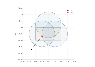
Convex projection of the intersection of convex sets using Dykstra’s algorithm.

Parameters:

projectionslist

A list of projection functions \(P_1, \ldots, P_m\).

niterint, optional

Maximum number of iterations.

tolfloat, optional

Tolerance on change of the solution (used as stopping criterion). If tol=0, run until niter is reached.

use_parallelbool, optional

If True, use the parallel version when $m=2$.

See also

pyproximal.projection.IntersectionProj

The convex projection onto the intersection of a particular type of convex sets.

pyproximal.GenericIntersectionProx

The corresponding indicator function.

pyproximal.Sum

Proximal operator of a sum of two or more convex functions using Dykstra-like algorithm.

Notes

Given a collection of convex projections \(P_i\) for \(i = 1, \ldots, m\), where each projection \(P_i(\mathbf{x})\) maps a point \(\mathbf{x}\) onto the convex set \(C_i\), the overall projection \(P_C(\mathbf{x})\) of \(\mathbf{x}\) onto the intersection of such sets \(C = \cap_{i=1}^m C_i\) is computed using the Dykstra’s algorithm. (\(C\) should not be empty.)

For \(m=2\), the projection \(P_C(\mathbf{x})\) of \(\mathbf{x}\) is computed by the Dykstra’s algorithm [1], [2], [3]:

• \(\mathbf{x}^0 = \mathbf{x}, \mathbf{p}^0 = \mathbf{q}^0 = 0\),

• for \(k = 1, \ldots\)

  • \(\mathbf{y}^k = P_1(\mathbf{x}^k + \mathbf{p}^k)\)

  • \(\mathbf{p}^{k+1} = \mathbf{x}^k + \mathbf{p}^k - \mathbf{y}^k\)

  • \(\mathbf{x}^{k+1} = P_2(\mathbf{y}^k + \mathbf{q}^k)\)

  • \(\mathbf{q}^{k+1} = \mathbf{y}^k + \mathbf{q}^k - \mathbf{x}^{k+1}\)

For \(m \ge 2\), the projection \(P_C(\mathbf{x})\) is computed by the parallel Dykstra’s algorithm [5], [6]. The following is taken from [4]:

• \(\mathbf{u}_m^0 = \mathbf{x}, \mathbf{z}_1^0 = \cdots = \mathbf{z}_m^0 = 0\),

• for \(k = 1, \ldots\)

  • \(\mathbf{u}_0^k = \mathbf{u}_m^{k-1}\)

  • for \(i = 1, \ldots, m\)

    • \(\mathbf{u}_i^k = P_i(\mathbf{u}_{i-1}^k + \mathbf{z}_i^{k-1})\)

    • \(\mathbf{z}_i^k = \mathbf{z}_i^{k-1} + \mathbf{u}_{i-1}^k - \mathbf{u}_i^k\)

Note the this is the proximal operator of the corresponding indicator function (see pyproximal.GenericIntersectionProx for details).

References

[1]

Bauschke, H.H., Borwein, J.M., 1994. Dykstra’s Alternating Projection Algorithm for Two Sets. Journal of Approximation Theory 79, 418-443. https://doi.org/10.1006/jath.1994.1136 https://cmps-people.ok.ubc.ca/bauschke/Research/02.pdf

[2]

Bauschke, H.H., Burachik, R.S., Herman, D.B., Kaya, C.Y., 2020. On Dykstra’s algorithm: finite convergence, stalling, and the method of alternating projections. Optim Lett 14, 1975-1987. https://doi.org/10.1007/s11590-020-01600-4 https://arxiv.org/abs/2001.06747

[3]

Wikipedia, Dykstra’s projection algorithm. https://en.wikipedia.org/wiki/Dykstra%27s_projection_algorithm

[4]

Tibshirani, R.J., 2017. Dykstra’s Algorithm, ADMM, and Coordinate Descent: Connections, Insights, and Extensions, NeurIPS2017. Eq.(4). https://proceedings.neurips.cc/paper_files/paper/2017/hash/5ef698cd9fe650923ea331c15af3b160-Abstract.html

[5]

Bauschke, H.H., Combettes, P.L., 2011. Convex Analysis and Monotone Operator Theory in Hilbert Spaces, Theorem 29.2, 1st ed, Springer. https://doi.org/10.1007/978-1-4419-9467-7

[6]

Bauschke, H.H., Lewis, A.S., 2000. Dykstras algorithm with bregman projections: A convergence proof. Optimization 48, 409-427. https://doi.org/10.1080/02331930008844513 https://people.orie.cornell.edu/aslewis/publications/00-dykstras.pdf

Methods

__init__(projections[, niter, tol, use_parallel])

Examples using pyproximal.projection.GenericIntersectionProj

Dykstra’s algorithms

Dykstra's algorithms