Note
Go to the end to download the full example code.
Low-Rank completion via Matrix factorization
In this tutorial we will present another example of low-rank matrix completion. This time, however, we will not leverage SVD to find a low-rank representation of the matrix, instead we will look for two matrices whose inner product can represent the matrix we are after.
More specifically we will consider the following forward problem:
where the non-negativity constraint (\(\delta_{\cdot \ge0}\)) is simply implemented using a Box proximal operator.
import matplotlib.pyplot as plt
import numpy as np
import pylops

import pyproximal

plt.close("all")
np.random.seed(10)


def callback(x, y, n, m, k, xtrue, snr_hist):
    snr_hist.append(pylops.utils.metrics.snr(xtrue, x.reshape(n, k) @ y.reshape(k, m)))
Let’s start by creating the matrix we want to factorize
n, m, k = 100, 90, 10
X = np.maximum(np.random.normal(0, 1, (n, k)), 0) + 1.0
Y = np.maximum(np.random.normal(0, 1, (k, m)), 0) + 1.0

A = X @ Y
We can now define the Box operators and the Low-Rank factorized operator. To do so we need some initial guess of \(\mathbf{X}\) and \(\mathbf{Y}\) that we create using the same distribution of the original ones.
nn1 = pyproximal.Box(lower=0)
nn2 = pyproximal.Box(lower=0)

Xin = np.maximum(np.random.normal(0, 1, (n, k)), 0) + 1.0
Yin = np.maximum(np.random.normal(0, 1, (k, m)), 0) + 1.0
Hop = pyproximal.utils.bilinear.LowRankFactorizedMatrix(Xin, Yin, A.ravel())
We are now ready to run the PALM algorithm
snr_palm = []
Xpalm, Ypalm = pyproximal.optimization.palm.PALM(
Hop,
nn1,
nn2,
Xin.ravel(),
Yin.ravel(),
gammaf=2,
gammag=2,
niter=2000,
show=True,
callback=lambda x, y: callback(x, y, n, m, k, A, snr_palm),
)
Xpalm, Ypalm = Xpalm.reshape(Xin.shape), Ypalm.reshape(Yin.shape)
Apalm = Xpalm @ Ypalm
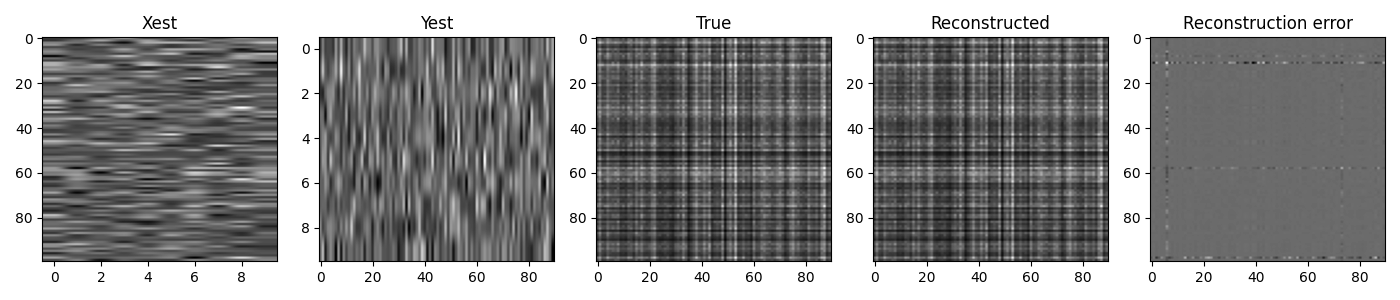
fig, axs = plt.subplots(1, 5, figsize=(14, 3))
fig.suptitle("PALM")
axs[0].imshow(Xpalm, cmap="gray")
axs[0].set_title("Xest")
axs[0].axis("tight")
axs[1].imshow(Ypalm, cmap="gray")
axs[1].set_title("Yest")
axs[1].axis("tight")
axs[2].imshow(A, cmap="gray", vmin=10, vmax=37)
axs[2].set_title("True")
axs[2].axis("tight")
axs[3].imshow(Apalm, cmap="gray", vmin=10, vmax=37)
axs[3].set_title("Reconstructed")
axs[3].axis("tight")
axs[4].imshow(A - Apalm, cmap="gray", vmin=-0.1, vmax=0.1)
axs[4].set_title("Reconstruction error")
axs[4].axis("tight")
fig.tight_layout()
PALM algorithm
---------------------------------------------------------
Bilinear operator: <class 'pyproximal.utils.bilinear.LowRankFactorizedMatrix'>
Proximal operator (f): <class 'pyproximal.proximal.Box.Box'>
Proximal operator (g): <class 'pyproximal.proximal.Box.Box'>
gammaf = 2      gammag = 2      niter = 2000

   Itn      x[0]       y[0]        f         g         H         ck         dk
     1  1.54505e+00  7.20e-01  1.00e+00  1.00e+00  3.76e+04  3.60e+03  3.72e+03
     2  1.58309e+00  5.86e-01  1.00e+00  1.00e+00  1.51e+04  3.56e+03  3.73e+03
     3  1.60203e+00  5.21e-01  1.00e+00  1.00e+00  9.35e+03  3.58e+03  3.74e+03
     4  1.61030e+00  4.92e-01  1.00e+00  1.00e+00  7.80e+03  3.59e+03  3.75e+03
     5  1.61340e+00  4.80e-01  1.00e+00  1.00e+00  7.32e+03  3.59e+03  3.75e+03
     6  1.61407e+00  4.77e-01  1.00e+00  1.00e+00  7.10e+03  3.59e+03  3.75e+03
     7  1.61360e+00  4.79e-01  1.00e+00  1.00e+00  6.96e+03  3.59e+03  3.75e+03
     8  1.61261e+00  4.83e-01  1.00e+00  1.00e+00  6.84e+03  3.59e+03  3.75e+03
     9  1.61137e+00  4.88e-01  1.00e+00  1.00e+00  6.73e+03  3.59e+03  3.75e+03
    10  1.61002e+00  4.94e-01  1.00e+00  1.00e+00  6.63e+03  3.59e+03  3.75e+03
   201  1.29414e+00  8.32e-01  1.00e+00  1.00e+00  2.65e+03  3.59e+03  3.75e+03
   401  9.24029e-01  7.10e-01  1.00e+00  1.00e+00  9.71e+02  3.59e+03  3.75e+03
   601  7.94781e-01  7.22e-01  1.00e+00  1.00e+00  3.89e+02  3.59e+03  3.76e+03
   801  7.68253e-01  7.50e-01  1.00e+00  1.00e+00  1.36e+02  3.58e+03  3.77e+03
  1001  7.73375e-01  7.53e-01  1.00e+00  1.00e+00  1.91e+01  3.58e+03  3.77e+03
  1201  7.77244e-01  7.52e-01  1.00e+00  1.00e+00  4.54e+00  3.57e+03  3.78e+03
  1401  7.81142e-01  7.50e-01  1.00e+00  1.00e+00  2.54e+00  3.57e+03  3.78e+03
  1601  7.85962e-01  7.48e-01  1.00e+00  1.00e+00  1.86e+00  3.56e+03  3.79e+03
  1801  7.91002e-01  7.45e-01  1.00e+00  1.00e+00  1.44e+00  3.56e+03  3.79e+03
  1992  7.95595e-01  7.42e-01  1.00e+00  1.00e+00  1.15e+00  3.56e+03  3.79e+03
  1993  7.95618e-01  7.42e-01  1.00e+00  1.00e+00  1.15e+00  3.56e+03  3.79e+03
  1994  7.95641e-01  7.42e-01  1.00e+00  1.00e+00  1.15e+00  3.56e+03  3.79e+03
  1995  7.95664e-01  7.42e-01  1.00e+00  1.00e+00  1.14e+00  3.56e+03  3.79e+03
  1996  7.95687e-01  7.42e-01  1.00e+00  1.00e+00  1.14e+00  3.56e+03  3.79e+03
  1997  7.95710e-01  7.42e-01  1.00e+00  1.00e+00  1.14e+00  3.56e+03  3.79e+03
  1998  7.95733e-01  7.42e-01  1.00e+00  1.00e+00  1.14e+00  3.56e+03  3.79e+03
  1999  7.95756e-01  7.42e-01  1.00e+00  1.00e+00  1.14e+00  3.56e+03  3.79e+03
  2000  7.95779e-01  7.42e-01  1.00e+00  1.00e+00  1.14e+00  3.56e+03  3.79e+03

Total time (s) = 0.21
---------------------------------------------------------
Similarly we run the PALM algorithm with backtracking
snr_palmbt = []
Xpalmbt, Ypalmbt = pyproximal.optimization.palm.PALM(
    Hop,
    nn1,
    nn2,
    Xin.ravel(),
    Yin.ravel(),
    gammaf=None,
    gammag=None,
    niter=2000,
    show=True,
    callback=lambda x, y: callback(x, y, n, m, k, A, snr_palmbt),
)
Xpalmbt, Ypalmbt = Xpalmbt.reshape(Xin.shape), Ypalmbt.reshape(Yin.shape)
Apalmbt = Xpalmbt @ Ypalmbt

fig, axs = plt.subplots(1, 5, figsize=(14, 3))
fig.suptitle("PALM with back-tracking")
axs[0].imshow(Xpalmbt, cmap="gray")
axs[0].set_title("Xest")
axs[0].axis("tight")
axs[1].imshow(Ypalmbt, cmap="gray")
axs[1].set_title("Yest")
axs[1].axis("tight")
axs[2].imshow(A, cmap="gray", vmin=10, vmax=37)
axs[2].set_title("True")
axs[2].axis("tight")
axs[3].imshow(Apalmbt, cmap="gray", vmin=10, vmax=37)
axs[3].set_title("Reconstructed")
axs[3].axis("tight")
axs[4].imshow(A - Apalmbt, cmap="gray", vmin=-0.1, vmax=0.1)
axs[4].set_title("Reconstruction error")
axs[4].axis("tight")
fig.tight_layout()

PALM algorithm
---------------------------------------------------------
Bilinear operator: <class 'pyproximal.utils.bilinear.LowRankFactorizedMatrix'>
Proximal operator (f): <class 'pyproximal.proximal.Box.Box'>
Proximal operator (g): <class 'pyproximal.proximal.Box.Box'>
gammaf = None   gammag = None   niter = 2000

   Itn      x[0]       y[0]        f         g         H         ck         dk
     1  1.59958e+00  4.70e-01  1.00e+00  1.00e+00  9.07e+03  0.00e+00  0.00e+00
     2  1.61385e+00  4.41e-01  1.00e+00  1.00e+00  7.41e+03  0.00e+00  0.00e+00
     3  1.61315e+00  4.50e-01  1.00e+00  1.00e+00  7.15e+03  0.00e+00  0.00e+00
     4  1.61075e+00  4.62e-01  1.00e+00  1.00e+00  6.94e+03  0.00e+00  0.00e+00
     5  1.60821e+00  4.73e-01  1.00e+00  1.00e+00  6.74e+03  0.00e+00  0.00e+00
     6  1.60572e+00  4.84e-01  1.00e+00  1.00e+00  6.55e+03  0.00e+00  0.00e+00
     7  1.60329e+00  4.95e-01  1.00e+00  1.00e+00  6.38e+03  0.00e+00  0.00e+00
     8  1.60091e+00  5.05e-01  1.00e+00  1.00e+00  6.23e+03  0.00e+00  0.00e+00
     9  1.59858e+00  5.15e-01  1.00e+00  1.00e+00  6.09e+03  0.00e+00  0.00e+00
    10  1.59629e+00  5.25e-01  1.00e+00  1.00e+00  5.95e+03  0.00e+00  0.00e+00
   201  9.68916e-01  7.23e-01  1.00e+00  1.00e+00  1.17e+03  0.00e+00  0.00e+00
   401  7.70347e-01  7.33e-01  1.00e+00  1.00e+00  2.08e+02  0.00e+00  0.00e+00
   601  7.75109e-01  7.35e-01  1.00e+00  1.00e+00  8.43e+00  0.00e+00  0.00e+00
   801  7.82535e-01  7.31e-01  1.00e+00  1.00e+00  2.05e+00  0.00e+00  0.00e+00
  1001  7.92735e-01  7.25e-01  1.00e+00  1.00e+00  1.24e+00  0.00e+00  0.00e+00
  1201  8.02248e-01  7.20e-01  1.00e+00  1.00e+00  8.26e-01  0.00e+00  0.00e+00
  1401  8.10134e-01  7.16e-01  1.00e+00  1.00e+00  5.68e-01  0.00e+00  0.00e+00
  1601  8.16493e-01  7.12e-01  1.00e+00  1.00e+00  4.03e-01  0.00e+00  0.00e+00
  1801  8.21586e-01  7.10e-01  1.00e+00  1.00e+00  2.93e-01  0.00e+00  0.00e+00
  1992  8.25497e-01  7.08e-01  1.00e+00  1.00e+00  2.20e-01  0.00e+00  0.00e+00
  1993  8.25516e-01  7.08e-01  1.00e+00  1.00e+00  2.20e-01  0.00e+00  0.00e+00
  1994  8.25534e-01  7.08e-01  1.00e+00  1.00e+00  2.20e-01  0.00e+00  0.00e+00
  1995  8.25552e-01  7.08e-01  1.00e+00  1.00e+00  2.19e-01  0.00e+00  0.00e+00
  1996  8.25571e-01  7.08e-01  1.00e+00  1.00e+00  2.19e-01  0.00e+00  0.00e+00
  1997  8.25589e-01  7.08e-01  1.00e+00  1.00e+00  2.19e-01  0.00e+00  0.00e+00
  1998  8.25607e-01  7.08e-01  1.00e+00  1.00e+00  2.18e-01  0.00e+00  0.00e+00
  1999  8.25626e-01  7.08e-01  1.00e+00  1.00e+00  2.18e-01  0.00e+00  0.00e+00
  2000  8.25644e-01  7.08e-01  1.00e+00  1.00e+00  2.18e-01  0.00e+00  0.00e+00

Total time (s) = 0.31
---------------------------------------------------------
And the iPALM algorithm
snr_ipalm = []
Xipalm, Yipalm = pyproximal.optimization.palm.iPALM(
    Hop,
    nn1,
    nn2,
    Xin.ravel(),
    Yin.ravel(),
    gammaf=2,
    gammag=2,
    a=[0.8, 0.8],
    niter=2000,
    show=True,
    callback=lambda x, y: callback(x, y, n, m, k, A, snr_ipalm),
)
Xipalm, Yipalm = Xipalm.reshape(Xin.shape), Yipalm.reshape(Yin.shape)
Aipalm = Xipalm @ Yipalm

fig, axs = plt.subplots(1, 5, figsize=(14, 3))
fig.suptitle("iPALM")
axs[0].imshow(Xipalm, cmap="gray")
axs[0].set_title("Xest")
axs[0].axis("tight")
axs[1].imshow(Yipalm, cmap="gray")
axs[1].set_title("Yest")
axs[1].axis("tight")
axs[2].imshow(A, cmap="gray", vmin=10, vmax=37)
axs[2].set_title("True")
axs[2].axis("tight")
axs[3].imshow(Aipalm, cmap="gray", vmin=10, vmax=37)
axs[3].set_title("Reconstructed")
axs[3].axis("tight")
axs[4].imshow(A - Aipalm, cmap="gray", vmin=-0.1, vmax=0.1)
axs[4].set_title("Reconstruction error")
axs[4].axis("tight")
fig.tight_layout()

iPALM algorithm
---------------------------------------------------------
Bilinear operator: <class 'pyproximal.utils.bilinear.LowRankFactorizedMatrix'>
Proximal operator (f): <class 'pyproximal.proximal.Box.Box'>
Proximal operator (g): <class 'pyproximal.proximal.Box.Box'>
gammaf = 2      gammag = 2
a = [0.8, 0.8]  niter = 2000

   Itn      x[0]       y[0]        f         g         H         ck         dk
     1  1.55607e+00  7.09e-01  1.00e+00  1.00e+00  3.83e+04  3.60e+03  3.84e+03
     2  1.61326e+00  4.58e-01  1.00e+00  1.00e+00  7.90e+03  3.51e+03  3.82e+03
     3  1.63773e+00  3.55e-01  1.00e+00  1.00e+00  9.92e+03  3.51e+03  3.85e+03
     4  1.63135e+00  3.72e-01  1.00e+00  1.00e+00  9.83e+03  3.52e+03  3.85e+03
     5  1.61221e+00  4.41e-01  1.00e+00  1.00e+00  7.24e+03  3.51e+03  3.84e+03
     6  1.59446e+00  5.08e-01  1.00e+00  1.00e+00  6.08e+03  3.51e+03  3.84e+03
     7  1.58265e+00  5.52e-01  1.00e+00  1.00e+00  5.80e+03  3.51e+03  3.84e+03
     8  1.57554e+00  5.76e-01  1.00e+00  1.00e+00  5.52e+03  3.51e+03  3.84e+03
     9  1.57050e+00  5.91e-01  1.00e+00  1.00e+00  5.20e+03  3.51e+03  3.84e+03
    10  1.56561e+00  6.05e-01  1.00e+00  1.00e+00  4.95e+03  3.51e+03  3.84e+03
   201  7.95603e-01  7.28e-01  1.00e+00  1.00e+00  8.08e+00  3.50e+03  3.85e+03
   401  8.08535e-01  7.26e-01  1.00e+00  1.00e+00  9.53e-01  3.50e+03  3.86e+03
   601  8.20724e-01  7.18e-01  1.00e+00  1.00e+00  3.48e-01  3.50e+03  3.86e+03
   801  8.27577e-01  7.14e-01  1.00e+00  1.00e+00  1.54e-01  3.49e+03  3.86e+03
  1001  8.31325e-01  7.12e-01  1.00e+00  1.00e+00  7.61e-02  3.49e+03  3.86e+03
  1201  8.33378e-01  7.10e-01  1.00e+00  1.00e+00  3.88e-02  3.49e+03  3.86e+03
  1401  8.34523e-01  7.09e-01  1.00e+00  1.00e+00  2.01e-02  3.49e+03  3.86e+03
  1601  8.35170e-01  7.09e-01  1.00e+00  1.00e+00  1.04e-02  3.49e+03  3.86e+03
  1801  8.35542e-01  7.08e-01  1.00e+00  1.00e+00  5.37e-03  3.49e+03  3.86e+03
  1992  8.35753e-01  7.08e-01  1.00e+00  1.00e+00  2.85e-03  3.49e+03  3.86e+03
  1993  8.35754e-01  7.08e-01  1.00e+00  1.00e+00  2.84e-03  3.49e+03  3.86e+03
  1994  8.35755e-01  7.08e-01  1.00e+00  1.00e+00  2.84e-03  3.49e+03  3.86e+03
  1995  8.35756e-01  7.08e-01  1.00e+00  1.00e+00  2.83e-03  3.49e+03  3.86e+03
  1996  8.35757e-01  7.08e-01  1.00e+00  1.00e+00  2.82e-03  3.49e+03  3.86e+03
  1997  8.35757e-01  7.08e-01  1.00e+00  1.00e+00  2.81e-03  3.49e+03  3.86e+03
  1998  8.35758e-01  7.08e-01  1.00e+00  1.00e+00  2.80e-03  3.49e+03  3.86e+03
  1999  8.35759e-01  7.08e-01  1.00e+00  1.00e+00  2.79e-03  3.49e+03  3.86e+03
  2000  8.35760e-01  7.08e-01  1.00e+00  1.00e+00  2.78e-03  3.49e+03  3.86e+03

Total time (s) = 0.22
---------------------------------------------------------
And finally compare the converge behaviour of the three methods
fig, ax = plt.subplots(1, 1, figsize=(8, 5))
ax.plot(snr_palm, "k", lw=2, label="PALM")
ax.plot(snr_palmbt, "r", lw=2, label="PALM-backtracking")
ax.plot(snr_ipalm, "g", lw=2, label="iPALM")
ax.grid()
ax.legend()
ax.set_title("SNR")
ax.set_xlabel("# Iteration")
fig.tight_layout()

Total running time of the script: (0 minutes 1.655 seconds)