Note
Go to the end to download the full example code.
Quadratic program with box constraints
This tutorial shows how we can use some of PyProximal solvers to solve a quadratic function with a box constraint:
More specifically we will consider both the
pyproximal.optimization.primal.ProximalGradient algorithm with and
without back-tracking.
In the literature you may find that problems of this kind can be solved by the so-called Projected Gradient Descent (PGD) algorithm: this is a edge case of a Proximal gradient solver when used with a constraint that admits a proximal (instead of a soft regularizer).
import matplotlib.pyplot as plt
import numpy as np
import pylops

import pyproximal

plt.close("all")
np.random.seed(10)
Let’s start defining the terms of the quadratic functional
We can now compute the functional within a grid, which we will show together with the evolution of the solution from the proximal gradient algorithm cost function grid
nm1, nm2 = 201, 201
m_min, m_max = (m[0] - 5, m[1] - 5), (m[0] + 5, m[1] + 5)
m1, m2 = np.linspace(m_min[0], m_max[0], nm1), np.linspace(m_min[1], m_max[1], nm2)
m1, m2 = np.meshgrid(m1, m2, indexing="ij")
mgrid = np.vstack((m1.ravel(), m2.ravel()))
J = 0.5 * np.sum(mgrid * np.dot(G, mgrid), axis=0) - np.dot(d, mgrid)
J = J.reshape(nm1, nm2)
We can now define the upper and lower bounds of the box and again we create a grid to display alongside the solution
We can now define both the quadratic functional and the box
l2 = pyproximal.L2(Op=pylops.MatrixMult(G), b=d, niter=2)
ind = pyproximal.Box(lower, upper)
We are now ready to solve our problem. All we need to do is to choose an initial guess for the proximal gradient algorithm
Provided we can estimate the spectral radius (i.e., max eigenvalue) of our
operator G, we can choose an optimal step and improve our convergence
speed.
Alternatively we can use back-tracking to adaptively find the best step at each iteration
mhist = [
    m0,
]
minv_back = pyproximal.optimization.primal.ProximalGradient(
    l2, ind, tau=None, x0=m0, epsg=1.0, niter=10, niterback=4, callback=callback
)
mhist_back = np.array(mhist)
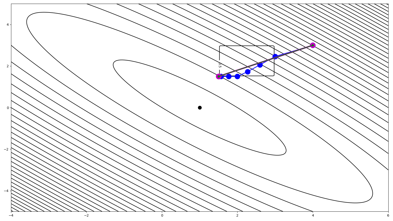
Finally let’s visualize the different trajectories and final solutions
fig, ax = plt.subplots(1, 1, figsize=(16, 9))
cs = ax.contour(m1, m2, J, levels=40, colors="k")
cs = ax.contour(m1, m2, indic, colors="k")
ax.clabel(cs, inline=1, fontsize=10)
ax.plot(m[0], m[1], ".k", ms=20)
ax.plot(m0[0], m0[1], ".r", ms=20)
ax.plot(mhist_slow[:, 0], mhist_slow[:, 1], ".-b", ms=30, lw=2)
ax.plot(mhist_opt[:, 0], mhist_opt[:, 1], ".-m", ms=30, lw=4)
ax.plot(mhist_back[:, 0], mhist_back[:, 1], ".-g", ms=10, lw=2)
plt.tight_layout()
Total running time of the script: (0 minutes 0.124 seconds)