Note
Go to the end to download the full example code.
Plug and Play Priors
In this tutorial we will consider a rather atypical proximal algorithm. In their seminal work, Venkatakrishnan et al. [2021], Plug-and-Play Priors for Model Based Reconstruction showed that the y-update in the ADMM algorithm can be interpreted as a denoising problem. The authors therefore suggested to replace the regularizer of the original problem with any denoising algorithm of choice (even if it does not have a known proximal). The proposed algorithm has shown great performance in a variety of inverse problems.
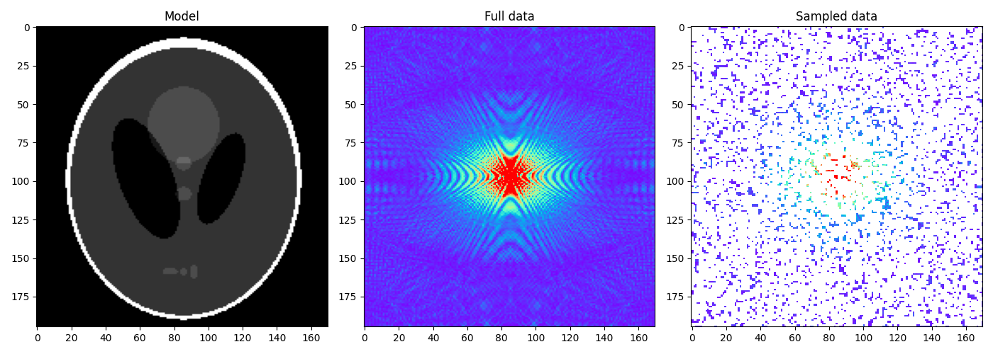
As an example, we will consider a simplified MRI experiment, where the data is created by appling a 2D Fourier Transform to the input model and by randomly sampling 60% of its values. We will use the famous BM3D as the denoiser, but any other denoiser of choice can be used instead!
Finally, whilst in the original paper, PnP is associated to the ADMM solver, subsequent
research showed that the same principle can be applied to pretty much any proximal
solver. We will show how to pass a solver of choice to our
pyproximal.optimization.pnp.PlugAndPlay solver.
import bm3d
import matplotlib.pyplot as plt
import numpy as np
import pylops
from pylops.config import set_ndarray_multiplication

import pyproximal

plt.close("all")
np.random.seed(0)
set_ndarray_multiplication(False)
Let’s start by loading the famous Shepp logan phantom and creating the modelling operator
x = np.load("../testdata/shepp_logan_phantom.npy")
x = x / x.max()
ny, nx = x.shape

perc_subsampling = 0.6
nxsub = int(np.round(ny * nx * perc_subsampling))
iava = np.sort(np.random.permutation(np.arange(ny * nx))[:nxsub])
Rop = pylops.Restriction(ny * nx, iava, dtype=np.complex128)
Fop = pylops.signalprocessing.FFT2D(dims=(ny, nx))
We now create and display the data alongside the model
y = Rop * Fop * x.ravel()
yfft = Fop * x.ravel()
yfft = np.fft.fftshift(yfft.reshape(ny, nx))

ymask = Rop.mask(Fop * x.ravel())
ymask = ymask.reshape(ny, nx)
ymask.data[:] = np.fft.fftshift(ymask.data)
ymask.mask[:] = np.fft.fftshift(ymask.mask)

fig, axs = plt.subplots(1, 3, figsize=(14, 5))
axs[0].imshow(x, vmin=0, vmax=1, cmap="gray")
axs[0].set_title("Model")
axs[0].axis("tight")
axs[1].imshow(np.abs(yfft), vmin=0, vmax=1, cmap="rainbow")
axs[1].set_title("Full data")
axs[1].axis("tight")
axs[2].imshow(np.abs(ymask), vmin=0, vmax=1, cmap="rainbow")
axs[2].set_title("Sampled data")
axs[2].axis("tight")
plt.tight_layout()
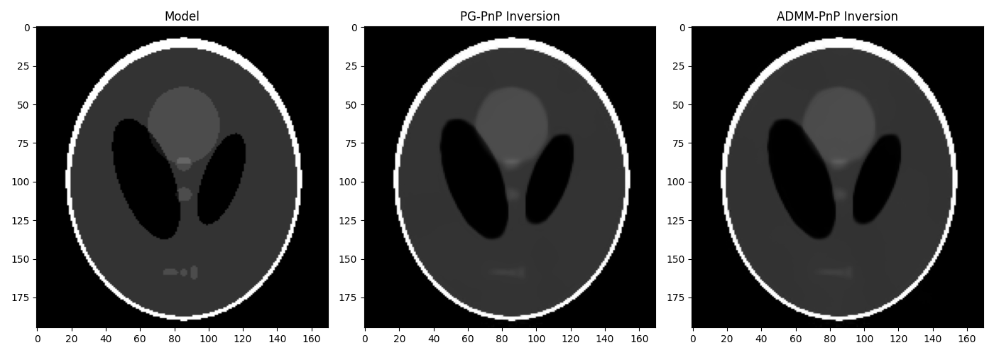
At this point we create a denoiser instance using the BM3D algorithm and use as Plug-and-Play Prior to the PG and ADMM algorithms
def callback(x, xtrue, errhist):
    errhist.append(np.linalg.norm(x - xtrue))


Op = Rop * Fop
L = np.real((Op.H * Op).eigs(neigs=1, which="LM")[0])
tau = 1.0 / L
sigma = 0.05

l2 = pyproximal.proximal.L2(Op=Op, b=y.ravel(), niter=50, warm=True)

# BM3D denoiser
denoiser = lambda x, tau: bm3d.bm3d(
    np.real(x), sigma_psd=sigma * tau, stage_arg=bm3d.BM3DStages.HARD_THRESHOLDING
)

# PG-Pnp
errhistpg = []
xpnppg = pyproximal.optimization.pnp.PlugAndPlay(
    l2,
    denoiser,
    x.shape,
    solver=pyproximal.optimization.primal.ProximalGradient,
    tau=tau,
    x0=np.zeros(x.size),
    niter=40,
    acceleration="fista",
    show=True,
    callback=lambda xx: callback(xx, x.ravel(), errhistpg),
)
xpnppg = np.real(xpnppg.reshape(x.shape))

# ADMM-PnP
errhistadmm = []
xpnpadmm = pyproximal.optimization.pnp.PlugAndPlay(
    l2,
    denoiser,
    x.shape,
    solver=pyproximal.optimization.primal.ADMM,
    tau=tau,
    x0=np.zeros(x.size),
    niter=40,
    show=True,
    callback=lambda xx: callback(xx, x.ravel(), errhistadmm),
)[0]
xpnpadmm = np.real(xpnpadmm.reshape(x.shape))

fig, axs = plt.subplots(1, 3, figsize=(14, 5))
axs[0].imshow(x, vmin=0, vmax=1, cmap="gray")
axs[0].set_title("Model")
axs[0].axis("tight")
axs[1].imshow(xpnppg, vmin=0, vmax=1, cmap="gray")
axs[1].set_title("PG-PnP Inversion")
axs[1].axis("tight")
axs[2].imshow(xpnpadmm, vmin=0, vmax=1, cmap="gray")
axs[2].set_title("ADMM-PnP Inversion")
axs[2].axis("tight")
plt.tight_layout()
Accelerated Proximal Gradient
---------------------------------------------------------
Proximal operator (f): <class 'pyproximal.proximal.L2.L2'>
Proximal operator (g): <class 'pyproximal.optimization.pnp._Denoise'>
tau = 0.9999999999999984        backtrack = False       beta = 5.000000e-01
epsg = 1.0      niter = 40      tol = None
niterback = 100 acceleration = fista

   Itn       x[0]          f           g       J=f+eps*g       tau
     1   5.79539e-02   6.093e+01   0.000e+00   6.093e+01   1.000e+00
     2   5.11582e-03   1.826e+01   0.000e+00   1.826e+01   1.000e+00
     3  -3.01890e-02   5.364e+00   0.000e+00   5.364e+00   1.000e+00
     4  -2.53920e-02   2.701e+00   0.000e+00   2.701e+00   1.000e+00
     5  -2.29824e-02   2.213e+00   0.000e+00   2.213e+00   1.000e+00
     6  -2.71790e-02   1.999e+00   0.000e+00   1.999e+00   1.000e+00
     7  -2.83003e-02   1.852e+00   0.000e+00   1.852e+00   1.000e+00
     8  -2.48831e-02   1.751e+00   0.000e+00   1.751e+00   1.000e+00
     9  -2.05380e-02   1.657e+00   0.000e+00   1.657e+00   1.000e+00
    10  -1.46019e-02   1.569e+00   0.000e+00   1.569e+00   1.000e+00
    13  -1.43390e-03   1.434e+00   0.000e+00   1.434e+00   1.000e+00
    17   2.77639e-04   1.404e+00   0.000e+00   1.404e+00   1.000e+00
    21  -2.18475e-03   1.411e+00   0.000e+00   1.411e+00   1.000e+00
    25  -4.27971e-03   1.421e+00   0.000e+00   1.421e+00   1.000e+00
    29  -3.73545e-03   1.423e+00   0.000e+00   1.423e+00   1.000e+00
    32  -2.78804e-03   1.421e+00   0.000e+00   1.421e+00   1.000e+00
    33  -2.74846e-03   1.416e+00   0.000e+00   1.416e+00   1.000e+00
    34  -2.69139e-03   1.415e+00   0.000e+00   1.415e+00   1.000e+00
    35  -2.65875e-03   1.412e+00   0.000e+00   1.412e+00   1.000e+00
    36  -2.75697e-03   1.412e+00   0.000e+00   1.412e+00   1.000e+00
    37  -2.92092e-03   1.416e+00   0.000e+00   1.416e+00   1.000e+00
    38  -2.98991e-03   1.420e+00   0.000e+00   1.420e+00   1.000e+00
    39  -3.07033e-03   1.421e+00   0.000e+00   1.421e+00   1.000e+00
    40  -3.24239e-03   1.420e+00   0.000e+00   1.420e+00   1.000e+00

Total time (s) = 24.33
---------------------------------------------------------

ADMM
---------------------------------------------------------
Proximal operator (f): <class 'pyproximal.proximal.L2.L2'>
Proximal operator (g): <class 'pyproximal.optimization.pnp._Denoise'>
tau = 1.000000e+00      niter = 40

   Itn       x[0]          f           g       J = f + g
     1   1.15604e-02   2.216e+02   0.000e+00   2.216e+02
     2  -8.56307e-03   1.145e+02   0.000e+00   1.145e+02
     3  -1.17574e-02   5.280e+01   0.000e+00   5.280e+01
     4  -2.08330e-02   2.375e+01   0.000e+00   2.375e+01
     5  -1.84653e-02   1.123e+01   0.000e+00   1.123e+01
     6  -1.71549e-02   6.032e+00   0.000e+00   6.032e+00
     7  -2.03437e-02   3.873e+00   0.000e+00   3.873e+00
     8  -2.14074e-02   2.922e+00   0.000e+00   2.922e+00
     9  -2.13936e-02   2.446e+00   0.000e+00   2.446e+00
    10  -2.20952e-02   2.195e+00   0.000e+00   2.195e+00
    13  -2.01355e-02   1.846e+00   0.000e+00   1.846e+00
    17  -1.56626e-02   1.628e+00   0.000e+00   1.628e+00
    21  -1.09523e-02   1.528e+00   0.000e+00   1.528e+00
    25  -8.01692e-03   1.469e+00   0.000e+00   1.469e+00
    29  -6.14493e-03   1.454e+00   0.000e+00   1.454e+00
    32  -5.21199e-03   1.440e+00   0.000e+00   1.440e+00
    33  -5.15385e-03   1.436e+00   0.000e+00   1.436e+00
    34  -4.66368e-03   1.438e+00   0.000e+00   1.438e+00
    35  -4.60660e-03   1.437e+00   0.000e+00   1.437e+00
    36  -4.48794e-03   1.437e+00   0.000e+00   1.437e+00
    37  -4.28470e-03   1.437e+00   0.000e+00   1.437e+00
    38  -4.17887e-03   1.428e+00   0.000e+00   1.428e+00
    39  -3.96370e-03   1.426e+00   0.000e+00   1.426e+00
    40  -4.15882e-03   1.424e+00   0.000e+00   1.424e+00

Total time (s) = 24.38
---------------------------------------------------------
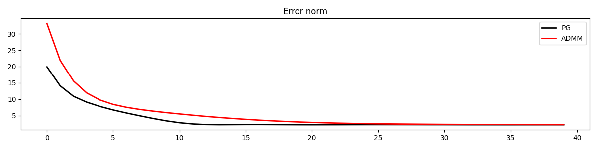
Finally, let’s compare the error convergence of the two variations of PnP
plt.figure(figsize=(12, 3))
plt.plot(errhistpg, "k", lw=2, label="PG")
plt.plot(errhistadmm, "r", lw=2, label="ADMM")
plt.title("Error norm")
plt.legend()
plt.tight_layout()
Total running time of the script: (0 minutes 49.429 seconds)