Note
Go to the end to download the full example code.
Basis Pursuit
This tutorial considers the Basis Pursuit problem. From a mathematical point of view we seek the sparsest solution that satisfies a system of equations.
where the operator \(\mathbf{A}\) is of size \(N \times M\), and generally \(N<M\). Note that this problem is similar to more general L1-regularized inversion, but it presents a stricter condition on the data term which must be satisfied exactly. Similarly, we can also consider the Basis Pursuit Denoise problem
import matplotlib.pyplot as plt
import numpy as np
import pylops

import pyproximal

plt.close("all")
np.random.seed(10)
Let’s start by creating the input vector x and operator A, and data y
This problem can be solved using the ADMM solver where f is an Affine set and g is the L1 norm
f = pyproximal.AffineSet(Aop, y, niter=20)
g = pyproximal.L1()
xinv_early = pyproximal.optimization.primal.ADMM(
f, g, np.zeros_like(x), 0.1, niter=10, show=True
)[0]
xinv = pyproximal.optimization.primal.ADMM(
f, g, np.zeros_like(x), 0.1, niter=150, show=True
)[0]
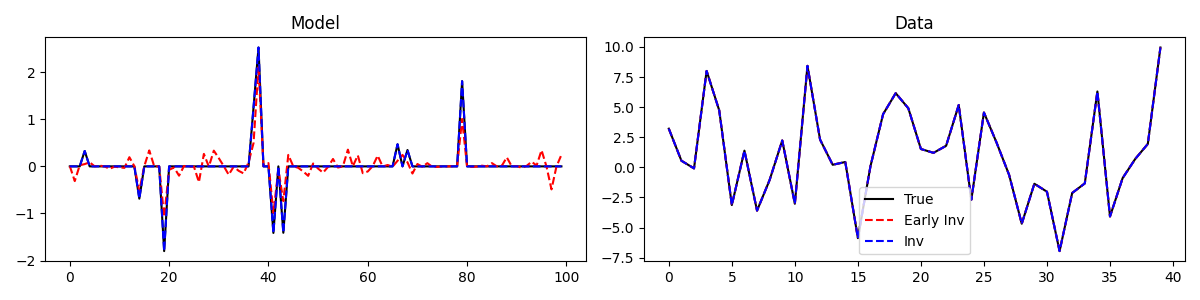
fig, axs = plt.subplots(1, 2, figsize=(12, 3))
axs[0].plot(x, "k")
axs[0].plot(xinv_early, "--r")
axs[0].plot(xinv, "--b")
axs[0].set_title("Model")
axs[1].plot(y, "k", label="True")
axs[1].plot(Aop * xinv_early, "--r", label="Early Inv")
axs[1].plot(Aop * xinv, "--b", label="Inv")
axs[1].set_title("Data")
axs[1].legend()
plt.tight_layout()
ADMM
---------------------------------------------------------
Proximal operator (f): <class 'pyproximal.proximal.AffineSet.AffineSet'>
Proximal operator (g): <class 'pyproximal.proximal.L1.L1'>
tau = 1.000000e-01      niter = 10

   Itn       x[0]          f           g       J = f + g
     1  -1.48208e-01   0.000e+00   1.979e+01   1.979e+01
     2  -1.17824e-01   0.000e+00   1.716e+01   1.716e+01
     3  -1.04548e-01   0.000e+00   1.667e+01   1.667e+01
     4  -7.88774e-02   0.000e+00   1.627e+01   1.627e+01
     5  -3.42487e-02   0.000e+00   1.598e+01   1.598e+01
     6   1.10090e-02   0.000e+00   1.558e+01   1.558e+01
     7   4.01171e-02   0.000e+00   1.531e+01   1.531e+01
     8   2.07255e-02   0.000e+00   1.520e+01   1.520e+01
     9   1.29133e-02   0.000e+00   1.496e+01   1.496e+01
    10   6.58063e-03   0.000e+00   1.463e+01   1.463e+01

Total time (s) = 0.00
---------------------------------------------------------

ADMM
---------------------------------------------------------
Proximal operator (f): <class 'pyproximal.proximal.AffineSet.AffineSet'>
Proximal operator (g): <class 'pyproximal.proximal.L1.L1'>
tau = 1.000000e-01      niter = 150

   Itn       x[0]          f           g       J = f + g
     1  -1.48208e-01   0.000e+00   1.979e+01   1.979e+01
     2  -1.17824e-01   0.000e+00   1.716e+01   1.716e+01
     3  -1.04548e-01   0.000e+00   1.667e+01   1.667e+01
     4  -7.88774e-02   0.000e+00   1.627e+01   1.627e+01
     5  -3.42487e-02   0.000e+00   1.598e+01   1.598e+01
     6   1.10090e-02   0.000e+00   1.558e+01   1.558e+01
     7   4.01171e-02   0.000e+00   1.531e+01   1.531e+01
     8   2.07255e-02   0.000e+00   1.520e+01   1.520e+01
     9   1.29133e-02   0.000e+00   1.496e+01   1.496e+01
    10   6.58063e-03   0.000e+00   1.463e+01   1.463e+01
    16  -1.66119e-03   0.000e+00   1.368e+01   1.368e+01
    31  -4.17020e-03   0.000e+00   1.250e+01   1.250e+01
    46   1.95677e-04   0.000e+00   1.209e+01   1.209e+01
    61   1.07793e-04   0.000e+00   1.205e+01   1.205e+01
    76   4.61062e-07   0.000e+00   1.204e+01   1.204e+01
    91   1.77417e-07   0.000e+00   1.204e+01   1.204e+01
   106   6.46170e-07   0.000e+00   1.203e+01   1.203e+01
   121   4.57747e-07   0.000e+00   1.203e+01   1.203e+01
   136   4.28310e-07   0.000e+00   1.203e+01   1.203e+01
   142   4.38472e-07   0.000e+00   1.203e+01   1.203e+01
   143   4.39766e-07   0.000e+00   1.203e+01   1.203e+01
   144   4.39837e-07   0.000e+00   1.203e+01   1.203e+01
   145   4.38918e-07   0.000e+00   1.203e+01   1.203e+01
   146   4.37419e-07   0.000e+00   1.203e+01   1.203e+01
   147   4.35799e-07   0.000e+00   1.203e+01   1.203e+01
   148   4.34448e-07   0.000e+00   1.203e+01   1.203e+01
   149   4.33615e-07   0.000e+00   1.203e+01   1.203e+01
   150   4.33383e-07   0.000e+00   1.203e+01   1.203e+01

Total time (s) = 0.05
---------------------------------------------------------
We can observe how even after few iterations, despite the solution is not yet converged the data reconstruction is perfect. This is consequence of the fact that for the Basis Pursuit problem the data term is a hard constraint. Finally let’s consider the case with a soft constraint.
f = pyproximal.L1()
g = pyproximal.proximal.EuclideanBall(y, 0.1)

L = np.real((Aop.H @ Aop).eigs(1))[0]
tau = 0.99
mu = tau / L

xinv_early = pyproximal.optimization.primaldual.PrimalDual(
    f, g, Aop, np.zeros_like(x), tau, mu, niter=10
)

xinv = pyproximal.optimization.primaldual.PrimalDual(
    f, g, Aop, np.zeros_like(x), tau, mu, niter=1000
)

fig, axs = plt.subplots(1, 2, figsize=(12, 3))
axs[0].plot(x, "k")
axs[0].plot(xinv_early, "--r")
axs[0].plot(xinv, "--b")
axs[0].set_title("Model")
axs[1].plot(y, "k", label="True")
axs[1].plot(Aop * xinv_early, "--r", label="Early Inv")
axs[1].plot(Aop * xinv, "--b", label="Inv (Res=%.2f)" % np.linalg.norm(y - Aop @ xinv))
axs[1].set_title("Data")
axs[1].legend()
plt.tight_layout()
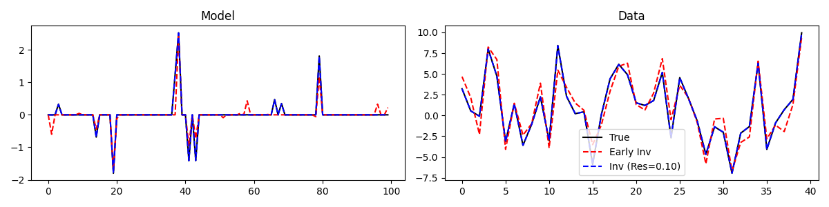
Note that at convergence the norm of the residual of the solution adheres to the EuclideanBall constraint
Total running time of the script: (0 minutes 0.349 seconds)