Note
Go to the end to download the full example code.
Denoising
This tutorial considers the classical problem of denoising of images affected by either random noise or salt-and-pepper noise using proximal algorithms.
The overall cost function to minimize is written in the following form:
where the L2 norm in the data term can be replaced by a L1 norm for salt-and-pepper (outlier like noise).
For both examples we investigate with different choices of regularization:
L2 on Gradient \(J(\mathbf{u}) = \|\nabla \mathbf{u}\|_2^2\)
Anisotropic TV \(J(\mathbf{u}) = \|\nabla \mathbf{u}\|_1\)
Isotropic TV \(J(\mathbf{u}) = \|\nabla \mathbf{u}\|_{2,1}\)
import matplotlib.pyplot as plt
import numpy as np
import pylops
from scipy import datasets

import pyproximal

plt.close("all")
np.random.seed(10)
Let’s start by loading a sample image and adding some noise
We can now define a pylops.Gradient operator that we are going to
use for all regularizers
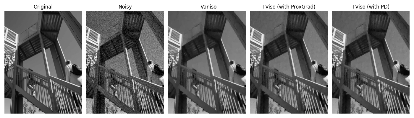
We then consider the first regularization (L2 norm on Gradient). We expect to get a smooth image where noise is suppressed by sharp edges in the original image are however lost.
# L2 data term
l2 = pyproximal.L2(b=noise_img.ravel())

# L2 regularization
sigma = 2.0
thik = pyproximal.L2(sigma=sigma)

# Solve
tau = 1.0
mu = 1.0 / (tau * L)

iml2 = pyproximal.optimization.primal.LinearizedADMM(
    l2, thik, Gop, tau=tau, mu=mu, x0=np.zeros_like(img.ravel()), niter=100
)[0]
iml2 = iml2.reshape(img.shape)
Let’s try now to use TV regularization, both anisotropic and isotropic
# L2 data term
l2 = pyproximal.L2(b=noise_img.ravel())

# Anisotropic TV
sigma = 0.1
l1 = pyproximal.L1(sigma=sigma)

# Solve
tau = 1.0
mu = tau / L

iml1 = pyproximal.optimization.primal.LinearizedADMM(
    l2, l1, Gop, tau=tau, mu=mu, x0=np.zeros_like(img.ravel()), niter=100
)[0]
iml1 = iml1.reshape(img.shape)


# Isotropic TV with Proximal Gradient
sigma = 0.1
tv = pyproximal.TV(dims=img.shape, sigma=sigma)

# Solve
tau = 1 / L

imtv = pyproximal.optimization.primal.ProximalGradient(
    l2, tv, tau=tau, x0=np.zeros_like(img.ravel()), niter=100
)
imtv = imtv.reshape(img.shape)

# Isotropic TV with Primal Dual
sigma = 0.1
l1iso = pyproximal.L21(ndim=2, sigma=sigma)

# Solve
tau = 1 / np.sqrt(L)
mu = 1.0 / (tau * L)

iml12 = pyproximal.optimization.primaldual.PrimalDual(
    l2, l1iso, Gop, tau=tau, mu=mu, theta=1.0, x0=np.zeros_like(img.ravel()), niter=100
)
iml12 = iml12.reshape(img.shape)

fig, axs = plt.subplots(1, 5, figsize=(14, 4))
axs[0].imshow(img, cmap="gray", vmin=0, vmax=1)
axs[0].set_title("Original")
axs[0].axis("off")
axs[0].axis("tight")
axs[1].imshow(noise_img, cmap="gray", vmin=0, vmax=1)
axs[1].set_title("Noisy")
axs[1].axis("off")
axs[1].axis("tight")
axs[2].imshow(iml1, cmap="gray", vmin=0, vmax=1)
axs[2].set_title("TVaniso")
axs[2].axis("off")
axs[2].axis("tight")
axs[3].imshow(imtv, cmap="gray", vmin=0, vmax=1)
axs[3].set_title("TViso (with ProxGrad)")
axs[3].axis("off")
axs[3].axis("tight")
axs[4].imshow(iml12, cmap="gray", vmin=0, vmax=1)
axs[4].set_title("TViso (with PD)")
axs[4].axis("off")
axs[4].axis("tight")
plt.tight_layout()
Finally we consider an example where the original image is corrupted by salt-and-pepper noise.
# Add salt and pepper noise
noiseperc = 0.1

isalt = np.random.permutation(np.arange(ny * nx))[: int(noiseperc * ny * nx)]
ipepper = np.random.permutation(np.arange(ny * nx))[: int(noiseperc * ny * nx)]
noise_img = img.copy().ravel()
noise_img[isalt] = img.max()
noise_img[ipepper] = img.min()
noise_img = noise_img.reshape(ny, nx)
Here we compare L2 and L1 norms for the data term L2 data term
l2 = pyproximal.L2(b=noise_img.ravel())

# L1 regularization (isotropic TV)
sigma = 0.2
l1iso = pyproximal.L21(ndim=2, sigma=sigma)

# Solve
tau = 0.1
mu = 1.0 / (tau * L)

iml12_l2 = pyproximal.optimization.primaldual.PrimalDual(
    l2,
    l1iso,
    Gop,
    tau=tau,
    mu=mu,
    theta=1.0,
    x0=np.zeros_like(noise_img).ravel(),
    niter=100,
    show=True,
)
iml12_l2 = iml12_l2.reshape(img.shape)


# L1 data term
l1 = pyproximal.L1(g=noise_img.ravel())

# L1 regularization (isotropic TV)
sigma = 0.7
l1iso = pyproximal.L21(ndim=2, sigma=sigma)

# Solve
tau = 1.0
mu = 1.0 / (tau * L)

iml12_l1 = pyproximal.optimization.primaldual.PrimalDual(
    l1,
    l1iso,
    Gop,
    tau=tau,
    mu=mu,
    theta=1.0,
    x0=np.zeros_like(noise_img).ravel(),
    niter=100,
    show=True,
)
iml12_l1 = iml12_l1.reshape(img.shape)

fig, axs = plt.subplots(2, 2, figsize=(14, 14))
axs[0][0].imshow(img, cmap="gray", vmin=0, vmax=1)
axs[0][0].set_title("Original")
axs[0][0].axis("off")
axs[0][0].axis("tight")
axs[0][1].imshow(noise_img, cmap="gray", vmin=0, vmax=1)
axs[0][1].set_title("Noisy")
axs[0][1].axis("off")
axs[0][1].axis("tight")
axs[1][0].imshow(iml12_l2, cmap="gray", vmin=0, vmax=1)
axs[1][0].set_title("L2data + TViso")
axs[1][0].axis("off")
axs[1][0].axis("tight")
axs[1][1].imshow(iml12_l1, cmap="gray", vmin=0, vmax=1)
axs[1][1].set_title("L1data + TViso")
axs[1][1].axis("off")
axs[1][1].axis("tight")
plt.tight_layout()
Primal-dual: min_x f(Ax) + x^T z + g(x)
---------------------------------------------------------
Proximal operator (f): <class 'pyproximal.proximal.L2.L2'>
Proximal operator (g): <class 'pyproximal.proximal.L21.L21'>
Linear operator (A): <class 'pylops.basicoperators.gradient.Gradient'>
Additional vector (z): None
tau = 0.1               mu = 1.25
theta = 1.00            niter = 100

   Itn       x[0]          f           g          z^x       J = f + g + z^x
     1   2.95900e-02   2.328e+04   1.472e+03   0.000e+00       2.475e+04
     2   5.64090e-02   2.020e+04   1.650e+03   0.000e+00       2.185e+04
     3   8.06757e-02   1.778e+04   1.601e+03   0.000e+00       1.938e+04
     4   1.00579e-01   1.579e+04   1.550e+03   0.000e+00       1.734e+04
     5   1.15844e-01   1.413e+04   1.532e+03   0.000e+00       1.566e+04
     6   1.27792e-01   1.275e+04   1.536e+03   0.000e+00       1.429e+04
     7   1.38069e-01   1.160e+04   1.550e+03   0.000e+00       1.315e+04
     8   1.47743e-01   1.063e+04   1.571e+03   0.000e+00       1.221e+04
     9   1.57141e-01   9.829e+03   1.596e+03   0.000e+00       1.143e+04
    10   1.66132e-01   9.159e+03   1.623e+03   0.000e+00       1.078e+04
    11   1.74477e-01   8.600e+03   1.649e+03   0.000e+00       1.025e+04
    21   2.37885e-01   6.246e+03   1.821e+03   0.000e+00       8.067e+03
    31   2.88518e-01   5.840e+03   1.887e+03   0.000e+00       7.727e+03
    41   2.96342e-01   5.758e+03   1.912e+03   0.000e+00       7.669e+03
    51   3.00095e-01   5.737e+03   1.920e+03   0.000e+00       7.657e+03
    61   3.02516e-01   5.731e+03   1.923e+03   0.000e+00       7.654e+03
    71   3.02892e-01   5.729e+03   1.923e+03   0.000e+00       7.652e+03
    81   3.03406e-01   5.728e+03   1.923e+03   0.000e+00       7.651e+03
    91   3.03612e-01   5.728e+03   1.923e+03   0.000e+00       7.651e+03
    92   3.03611e-01   5.728e+03   1.923e+03   0.000e+00       7.650e+03
    93   3.03609e-01   5.728e+03   1.923e+03   0.000e+00       7.650e+03
    94   3.03604e-01   5.728e+03   1.923e+03   0.000e+00       7.650e+03
    95   3.03598e-01   5.728e+03   1.923e+03   0.000e+00       7.650e+03
    96   3.03590e-01   5.728e+03   1.922e+03   0.000e+00       7.650e+03
    97   3.03582e-01   5.728e+03   1.922e+03   0.000e+00       7.650e+03
    98   3.03573e-01   5.728e+03   1.922e+03   0.000e+00       7.650e+03
    99   3.03564e-01   5.728e+03   1.922e+03   0.000e+00       7.650e+03
   100   3.03557e-01   5.728e+03   1.922e+03   0.000e+00       7.650e+03

Total time (s) = 1.23
---------------------------------------------------------

Primal-dual: min_x f(Ax) + x^T z + g(x)
---------------------------------------------------------
Proximal operator (f): <class 'pyproximal.proximal.L1.L1'>
Proximal operator (g): <class 'pyproximal.proximal.L21.L21'>
Linear operator (A): <class 'pylops.basicoperators.gradient.Gradient'>
Additional vector (z): None
tau = 1.0               mu = 0.125
theta = 1.00            niter = 100

   Itn       x[0]          f           g          z^x       J = f + g + z^x
     1   3.25490e-01   0.000e+00   5.666e+04   0.000e+00       5.666e+04
     2   3.25490e-01   0.000e+00   5.666e+04   0.000e+00       5.666e+04
     3   3.25490e-01   2.369e+03   5.116e+04   0.000e+00       5.353e+04
     4   3.25490e-01   9.065e+03   3.653e+04   0.000e+00       4.560e+04
     5   3.25490e-01   1.654e+04   2.690e+04   0.000e+00       4.344e+04
     6   3.25490e-01   2.168e+04   2.375e+04   0.000e+00       4.543e+04
     7   3.25490e-01   2.395e+04   2.112e+04   0.000e+00       4.507e+04
     8   3.25490e-01   2.437e+04   1.729e+04   0.000e+00       4.166e+04
     9   3.25490e-01   2.409e+04   1.466e+04   0.000e+00       3.875e+04
    10   3.25490e-01   2.381e+04   1.319e+04   0.000e+00       3.700e+04
    11   3.25490e-01   2.375e+04   1.209e+04   0.000e+00       3.584e+04
    21   3.25490e-01   2.477e+04   7.507e+03   0.000e+00       3.228e+04
    31   3.25490e-01   2.492e+04   6.804e+03   0.000e+00       3.172e+04
    41   3.25490e-01   2.497e+04   6.565e+03   0.000e+00       3.153e+04
    51   3.25490e-01   2.499e+04   6.432e+03   0.000e+00       3.142e+04
    61   3.25490e-01   2.501e+04   6.336e+03   0.000e+00       3.135e+04
    71   3.25490e-01   2.503e+04   6.266e+03   0.000e+00       3.129e+04
    81   3.25490e-01   2.503e+04   6.218e+03   0.000e+00       3.125e+04
    91   3.25490e-01   2.504e+04   6.172e+03   0.000e+00       3.121e+04
    92   3.25490e-01   2.504e+04   6.168e+03   0.000e+00       3.121e+04
    93   3.25490e-01   2.504e+04   6.163e+03   0.000e+00       3.121e+04
    94   3.25490e-01   2.505e+04   6.158e+03   0.000e+00       3.120e+04
    95   3.25490e-01   2.505e+04   6.153e+03   0.000e+00       3.120e+04
    96   3.25490e-01   2.505e+04   6.149e+03   0.000e+00       3.120e+04
    97   3.25490e-01   2.505e+04   6.146e+03   0.000e+00       3.120e+04
    98   3.25490e-01   2.505e+04   6.141e+03   0.000e+00       3.119e+04
    99   3.25490e-01   2.505e+04   6.137e+03   0.000e+00       3.119e+04
   100   3.25490e-01   2.505e+04   6.134e+03   0.000e+00       3.119e+04

Total time (s) = 1.25
---------------------------------------------------------
Total running time of the script: (0 minutes 19.624 seconds)