Note
Go to the end to download the full example code.
Adaptive Primal-Dual
This tutorial compares the traditional Chambolle-Pock Primal-dual algorithm with the Adaptive Primal-Dual Hybrid Gradient of Goldstein and co-authors.
By adaptively changing the step size in the primal and the dual directions, this algorithm shows faster convergence, which is of great importance for some of the problems that the Primal-Dual algorithm can solve - especially those with an expensive proximal operator.
For this example, we consider a simple denoising problem.
import matplotlib.pyplot as plt
import numpy as np
import pylops
from skimage.data import camera

import pyproximal

plt.close("all")
np.random.seed(10)


def callback(x, f, g, K, cost, xtrue, err):
    cost.append(f(x) + g(K.matvec(x)))
    err.append(np.linalg.norm(x - xtrue))
Let’s start by loading a sample image and adding some noise
We can now define a pylops.Gradient operator as well as the
different proximal operators to be passed to our solvers
# Gradient operator
sampling = 1.0
Gop = pylops.Gradient(
    dims=(ny, nx), sampling=sampling, edge=False, kind="forward", dtype="float64"
)
L = 8.0 / sampling**2  # maxeig(Gop^H Gop)

# L2 data term
lamda = 0.04
l2 = pyproximal.L2(b=noise_img.ravel(), sigma=lamda)

# L1 regularization (isotropic TV)
l1iso = pyproximal.L21(ndim=2)
To start, we solve our denoising problem with the original Primal-Dual algorithm
# Primal-dual
tau = 0.95 / np.sqrt(L)
mu = 0.95 / np.sqrt(L)

cost_fixed = []
err_fixed = []
iml12_fixed = pyproximal.optimization.primaldual.PrimalDual(
    l2,
    l1iso,
    Gop,
    tau=tau,
    mu=mu,
    theta=1.0,
    x0=np.zeros_like(img.ravel()),
    gfirst=False,
    niter=300,
    show=True,
    callback=lambda x: callback(x, l2, l1iso, Gop, cost_fixed, img.ravel(), err_fixed),
)
iml12_fixed = iml12_fixed.reshape(img.shape)
Primal-dual: min_x f(Ax) + x^T z + g(x)
---------------------------------------------------------
Proximal operator (f): <class 'pyproximal.proximal.L2.L2'>
Proximal operator (g): <class 'pyproximal.proximal.L21.L21'>
Linear operator (A): <class 'pylops.basicoperators.gradient.Gradient'>
Additional vector (z): None
tau = 0.33587572106361          mu = 0.33587572106361
theta = 1.00            niter = 300

   Itn       x[0]          f           g          z^x       J = f + g + z^x
     1   3.00444e+00   1.147e+08   1.330e+05   0.000e+00       1.148e+08
     2   5.81247e+00   1.117e+08   1.383e+05   0.000e+00       1.118e+08
     3   8.42311e+00   1.088e+08   1.217e+05   0.000e+00       1.090e+08
     4   1.08909e+01   1.060e+08   1.115e+05   0.000e+00       1.062e+08
     5   1.32918e+01   1.033e+08   1.108e+05   0.000e+00       1.034e+08
     6   1.56633e+01   1.007e+08   1.142e+05   0.000e+00       1.008e+08
     7   1.80377e+01   9.811e+07   1.186e+05   0.000e+00       9.823e+07
     8   2.04249e+01   9.560e+07   1.239e+05   0.000e+00       9.572e+07
     9   2.28176e+01   9.315e+07   1.302e+05   0.000e+00       9.328e+07
    10   2.51984e+01   9.077e+07   1.372e+05   0.000e+00       9.090e+07
    31   6.70586e+01   5.294e+07   2.872e+05   0.000e+00       5.323e+07
    61   1.11036e+02   2.517e+07   4.528e+05   0.000e+00       2.562e+07
    91   1.40073e+02   1.266e+07   5.656e+05   0.000e+00       1.322e+07
   121   1.59613e+02   7.017e+06   6.413e+05   0.000e+00       7.658e+06
   151   1.72686e+02   4.467e+06   6.921e+05   0.000e+00       5.159e+06
   181   1.81454e+02   3.311e+06   7.262e+05   0.000e+00       4.037e+06
   211   1.87322e+02   2.784e+06   7.490e+05   0.000e+00       3.533e+06
   241   1.91259e+02   2.543e+06   7.644e+05   0.000e+00       3.307e+06
   271   1.93895e+02   2.431e+06   7.746e+05   0.000e+00       3.206e+06
   292   1.95204e+02   2.390e+06   7.797e+05   0.000e+00       3.170e+06
   293   1.95258e+02   2.389e+06   7.800e+05   0.000e+00       3.169e+06
   294   1.95311e+02   2.387e+06   7.802e+05   0.000e+00       3.168e+06
   295   1.95363e+02   2.386e+06   7.804e+05   0.000e+00       3.166e+06
   296   1.95414e+02   2.385e+06   7.806e+05   0.000e+00       3.165e+06
   297   1.95465e+02   2.383e+06   7.808e+05   0.000e+00       3.164e+06
   298   1.95515e+02   2.382e+06   7.810e+05   0.000e+00       3.163e+06
   299   1.95565e+02   2.381e+06   7.811e+05   0.000e+00       3.162e+06
   300   1.95613e+02   2.380e+06   7.813e+05   0.000e+00       3.161e+06

Total time (s) = 5.53
---------------------------------------------------------
We do the same with the adaptive algorithm
cost_ada = []
err_ada = []
iml12_ada, steps = pyproximal.optimization.primaldual.AdaptivePrimalDual(
    l2,
    l1iso,
    Gop,
    tau=tau,
    mu=mu,
    x0=np.zeros_like(img.ravel()),
    niter=45,
    show=True,
    tol=0.05,
    callback=lambda x: callback(x, l2, l1iso, Gop, cost_ada, img.ravel(), err_ada),
)
iml12_ada = iml12_ada.reshape(img.shape)
Adaptive Primal-dual: min_x f(Ax) + x^T z + g(x)
---------------------------------------------------------
Proximal operator (f): <class 'pyproximal.proximal.L2.L2'>
Proximal operator (g): <class 'pyproximal.proximal.L21.L21'>
Linear operator (A): <class 'pylops.basicoperators.gradient.Gradient'>
Additional vector (z): None
tau0 = 3.358757e-01     mu0 = 3.358757e-01
alpha0 = 5.000000e-01   eta = 9.500000e-01
s = 1.000000e+00        delta = 1.500000e+00
niter = 45              tol = 5.000000e-02

   Itn       x[0]          f           g          z^x       J = f + g + z^x
     2   3.00444e+00   1.147e+08   1.330e+05   0.000e+00       1.148e+08
     3   8.54703e+00   1.088e+08   1.625e+05   0.000e+00       1.090e+08
     4   1.81498e+01   9.875e+07   2.030e+05   0.000e+00       9.895e+07
     5   3.38450e+01   8.305e+07   2.859e+05   0.000e+00       8.333e+07
     6   5.73664e+01   6.204e+07   4.075e+05   0.000e+00       6.245e+07
     7   8.85500e+01   3.910e+07   5.559e+05   0.000e+00       3.966e+07
     8   1.13090e+02   2.498e+07   6.642e+05   0.000e+00       2.565e+07
     9   1.32395e+02   1.629e+07   7.390e+05   0.000e+00       1.703e+07
    10   1.47554e+02   1.093e+07   7.898e+05   0.000e+00       1.172e+07
    13   1.73504e+02   4.728e+06   8.550e+05   0.000e+00       5.583e+06
    17   1.79673e+02   3.757e+06   8.434e+05   0.000e+00       4.600e+06
    21   1.82680e+02   3.307e+06   8.302e+05   0.000e+00       4.137e+06
    25   1.85647e+02   2.932e+06   8.401e+05   0.000e+00       3.772e+06
    29   1.87761e+02   2.697e+06   8.311e+05   0.000e+00       3.528e+06
    33   1.89263e+02   2.557e+06   8.139e+05   0.000e+00       3.371e+06
    37   1.90880e+02   2.471e+06   8.036e+05   0.000e+00       3.275e+06
    38   1.91304e+02   2.455e+06   8.020e+05   0.000e+00       3.257e+06
    39   1.91724e+02   2.441e+06   8.007e+05   0.000e+00       3.242e+06
    40   1.92137e+02   2.429e+06   7.997e+05   0.000e+00       3.229e+06
    41   1.92540e+02   2.418e+06   7.990e+05   0.000e+00       3.217e+06
    42   1.92931e+02   2.408e+06   7.984e+05   0.000e+00       3.206e+06
    43   1.93309e+02   2.399e+06   7.979e+05   0.000e+00       3.197e+06
    44   1.93675e+02   2.392e+06   7.976e+05   0.000e+00       3.189e+06
    45   1.94027e+02   2.385e+06   7.973e+05   0.000e+00       3.182e+06
    46   1.94365e+02   2.379e+06   7.970e+05   0.000e+00       3.176e+06

Total time (s) = 0.88
Let’s now compare the final results
fig, axs = plt.subplots(1, 4, figsize=(16, 4))
axs[0].imshow(img, cmap="gray", vmin=0, vmax=255)
axs[0].set_title("Original")
axs[0].axis("off")
axs[0].axis("tight")
axs[1].imshow(noise_img, cmap="gray", vmin=0, vmax=255)
axs[1].set_title("Noisy")
axs[1].axis("off")
axs[1].axis("tight")
axs[2].imshow(iml12_fixed, cmap="gray", vmin=0, vmax=255)
axs[2].set_title("PD")
axs[2].axis("off")
axs[2].axis("tight")
axs[3].imshow(iml12_ada, cmap="gray", vmin=0, vmax=255)
axs[3].set_title("Adaptive PD")
axs[3].axis("off")
axs[3].axis("tight")
plt.tight_layout()
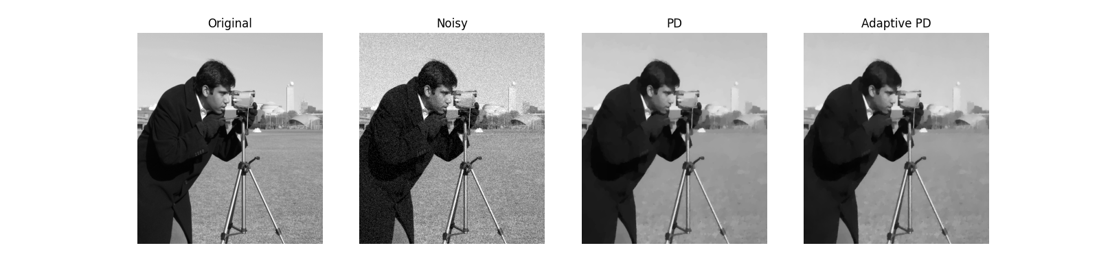
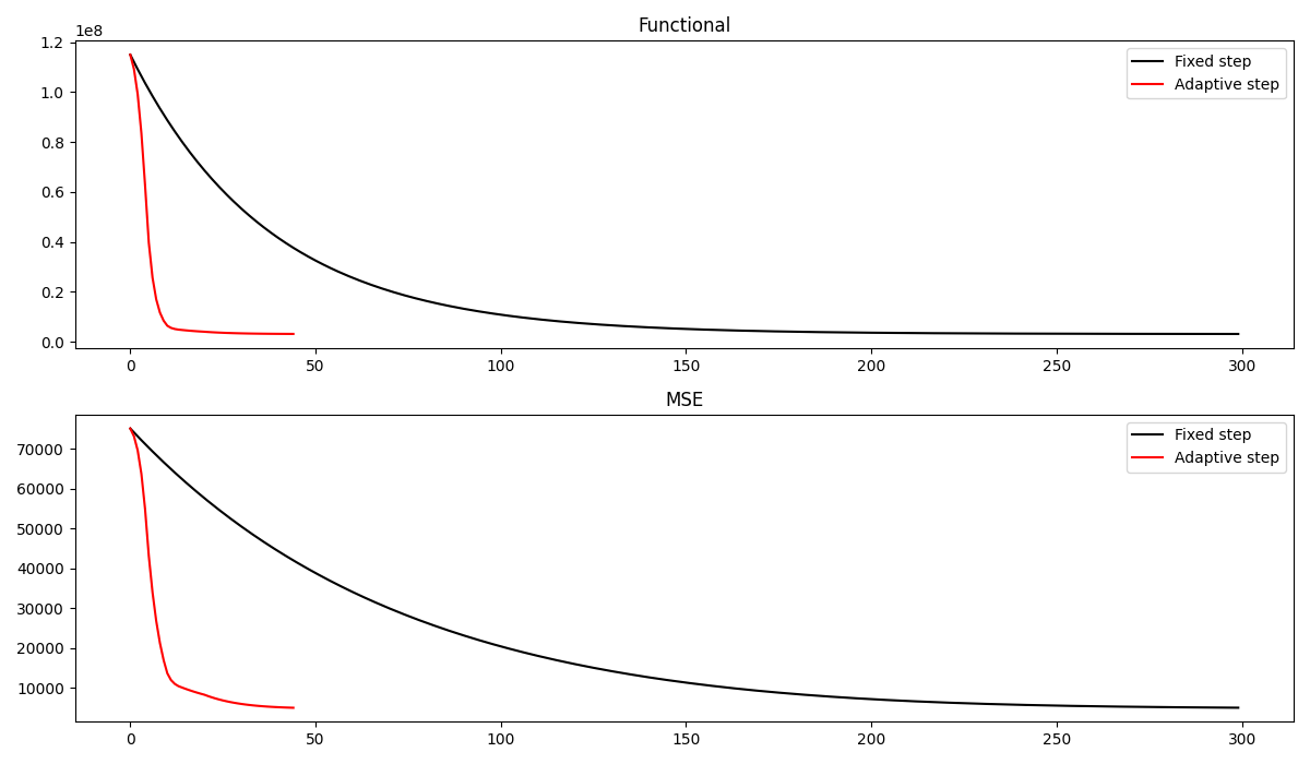
And the convergence curves of the two algorithms. We can see how the adaptive Primal-Dual produces a better estimate of the clean image in a much smaller number of iterations
fig, axs = plt.subplots(2, 1, figsize=(12, 7))
axs[0].plot(cost_fixed, "k", label="Fixed step")
axs[0].plot(cost_ada, "r", label="Adaptive step")
axs[0].legend()
axs[0].set_title("Functional")
axs[1].plot(err_fixed, "k", label="Fixed step")
axs[1].plot(err_ada, "r", label="Adaptive step")
axs[1].set_title("MSE")
axs[1].legend()
plt.tight_layout()
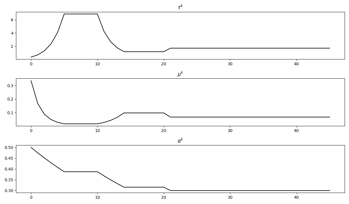
And to conclude we display the three different step sizes involved in the solver
Total running time of the script: (0 minutes 7.252 seconds)