pyproximal.optimization.primal.ProximalGradient
- pyproximal.optimization.primal.ProximalGradient(proxf: ProxOperator, proxg: ProxOperator, x0: ndarray[tuple[Any, ...], dtype[_ScalarT]], epsg: float | ndarray[tuple[Any, ...], dtype[_ScalarT]] = 1.0, tau: float | None = None, backtracking: bool = False, beta: float = 0.5, eta: float = 1.0, niter: int = 10, niterback: int = 100, acceleration: str | None = None, tol: float | None = None, callback: Callable[[ndarray[tuple[Any, ...], dtype[_ScalarT]]], None] | None = None, show: bool = False) ndarray[tuple[Any, ...], dtype[_ScalarT]][source]
Proximal gradient (optionally accelerated)
Solves the following minimization problem using (Accelerated) Proximal gradient algorithm:
\[\mathbf{x} = \argmin_\mathbf{x} f(\mathbf{x}) + \epsilon g(\mathbf{x})\]where \(f(\mathbf{x})\) is a smooth convex function with a uniquely defined gradient and \(g(\mathbf{x})\) is any convex function that has a known proximal operator.
- Parameters:
- proxf
pyproximal.ProxOperator Proximal operator of f function (must have
gradimplemented)- proxg
pyproximal.ProxOperator Proximal operator of g function
- x0
numpy.ndarray Initial vector
- epsg
floatornumpy.ndarray, optional Scaling factor of g function
- tau
floatornumpy.ndarray, optional Positive scalar weight, which should satisfy the following condition to guarantees convergence: \(\tau \in (0, 1/L]\) where
Lis the Lipschitz constant of \(\nabla f\). Whentau=None, backtracking is used to adaptively estimate the best tau at each iteration. Finally, note that \(\tau\) can be chosen to be a vector when dealing with problems with multiple right-hand-sides- backtracking
bool, optional Force backtracking, even if
tauis not equal toNone. In this case the chosentauwill be used as the initial guess in the first step of backtracking- beta
float, optional Backtracking parameter (must be between 0 and 1)
- eta
float, optional Relaxation parameter (must be between 0 and 1, 0 excluded).
- niter
int, optional Number of iterations of iterative scheme
- niterback
int, optional Max number of iterations of backtracking
- acceleration
str, optional Acceleration (
None,vandenbergheorfista)- tol
float, optional Tolerance on change of objective function (used as stopping criterion). If
tol=None, run untilniteris reached- callback
callable, optional Function with signature (
callback(x)) to call after each iteration wherexis the current model vector- show
bool, optional Display iterations log
- proxf
- Returns:
- x
numpy.ndarray Inverted model
- x
Notes
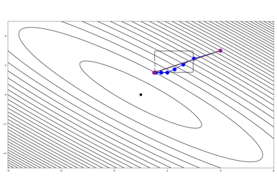
The Proximal gradient algorithm can be expressed by the following recursion:
\[\begin{split}\mathbf{x}^{k+1} = \mathbf{y}^k + \eta (\prox_{\tau^k \epsilon g}(\mathbf{y}^k - \tau^k \nabla f(\mathbf{y}^k)) - \mathbf{y}^k) \\ \mathbf{y}^{k+1} = \mathbf{x}^k + \omega^k (\mathbf{x}^k - \mathbf{x}^{k-1})\end{split}\]where at each iteration \(\tau^k\) can be estimated by back-tracking as follows:
\[\begin{split}\begin{aligned} &\tau = \tau^{k-1} &\\ &repeat \; \mathbf{z} = \prox_{\tau \epsilon g}(\mathbf{x}^k - \tau \nabla f(\mathbf{x}^k)), \tau = \beta \tau \quad if \; f(\mathbf{z}) \leq \tilde{f}_\tau(\mathbf{z}, \mathbf{x}^k) \\ &\tau^k = \tau, \quad \mathbf{x}^{k+1} = \mathbf{z} &\\ \end{aligned}\end{split}\]where \(\tilde{f}_\tau(\mathbf{x}, \mathbf{y}) = f(\mathbf{y}) + \nabla f(\mathbf{y})^T (\mathbf{x} - \mathbf{y}) + 1/(2\tau)||\mathbf{x} - \mathbf{y}||_2^2\).
Different accelerations are provided:
Examples using pyproximal.optimization.primal.ProximalGradient

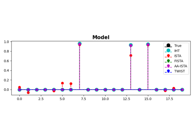
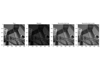
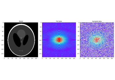
IHT, ISTA, FISTA, AA-ISTA, and TWIST for Compressive sensing