Relaxed Mumford-Shah regularization

In this tutorial we will use a relaxed Mumford-Shah (rMS) functional 1 as regularization, which has the following form:

\[\text{rMS}(x) = \min (\alpha\Vert x\Vert_2^2, \kappa).\]

Its corresponding proximal operator is given by

\[\begin{split}\text{prox}_{\tau \text{rMS}}(x) = \begin{cases} \frac{1}{1+2\tau \alpha}x & \text{ if } & \vert x\vert \leq \sqrt{\frac{\kappa}{\alpha}(1 + 2\tau \alpha)} \\ \kappa & \text{ else } \end{cases}.\end{split}\]

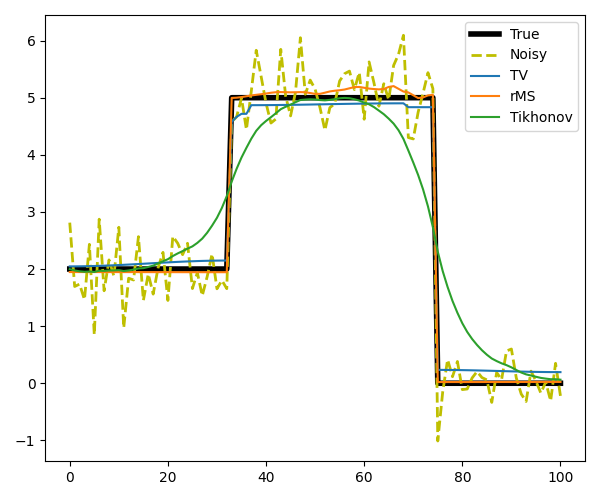
rMS is a combination of Tikhonov and TV regularization. Once the rMS hits a certain threshold, the solution will be allowed to jump due to the constant penalty \(\kappa\), and below this value rMS will be smooth due to Tikhonov regularization. We show three denoising examples: one example that is well-suited for TV regularization and two examples where rMS outperforms TV and Tikhonov regularization, modeled after the experiments in 2.

References

1

Strekalovskiy, E., and D. Cremers, 2014, Real-time minimization of the piecewise smooth Mumford-Shah functional: European Conference on Computer Vision, 127–141

2

Kadu, A., and Kumar, R. and van Leeuwen, Tristan. Full-waveform inversion with Mumford-Shah regularization. SEG International Exposition and Annual Meeting, SEG-2018-2997224

import numpy as np
import matplotlib.pyplot as plt
import pylops
import pyproximal

np.random.seed(1)

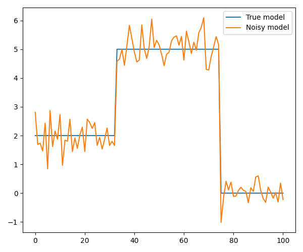
We start with a simple model with two jumps that is well-suited for TV regularization

# Create noisy data
nx = 101
idx_jump1 = nx // 3
idx_jump2 = 3 * nx // 4
x = np.zeros(nx)
x[:idx_jump1] = 2
x[idx_jump1:idx_jump2] = 5
n = np.random.normal(0, 0.5, nx)
y = x + n

# Plot the model and the noisy data
fig, axs = plt.subplots(1, 1, figsize=(6, 5))
axs.plot(x, label='True model')
axs.plot(y, label='Noisy model')
axs.legend()
plt.tight_layout()

For both rMS and TV regularizations we use the Linearized ADMM, whilst for Tikhonov regularization we use LSQR

# Define functionals
l2 = pyproximal.proximal.L2(b=y)
l1 = pyproximal.proximal.L1(sigma=5.)
Dop = pylops.FirstDerivative(nx, edge=True, kind='backward')

# TV
L = np.real((Dop.H * Dop).eigs(neigs=1, which='LM')[0])
tau = 1.
mu = 0.99 * tau / L
xTV, _ = pyproximal.optimization.primal.LinearizedADMM(l2, l1, Dop, tau=tau, mu=mu,
                                                       x0=np.zeros_like(x), niter=200)

# rMS
sigma = 1e5
kappa = 1e0
ms_relaxed = pyproximal.proximal.RelaxedMumfordShah(sigma=sigma, kappa=kappa)
tau = 1.
mu = tau / L
xrMS, _ = pyproximal.optimization.primal.LinearizedADMM(l2, ms_relaxed, Dop, tau=tau, mu=mu,
                                                        x0=np.zeros_like(x), niter=200)

# Tikhonov
xTikhonov = pylops.optimization.leastsquares.regularized_inversion(Op=pylops.Identity(nx),
                                                                   Regs=[Dop, ], y=y,
                                                                   epsRs=[6e0, ])[0]

# Plot the results
fig, axs = plt.subplots(1, 1, figsize=(6, 5))
axs.plot(x, label='True', linewidth=4, color='k')
axs.plot(y, '--', label='Noisy', linewidth=2, color='y')
axs.plot(xTV, label='TV')
axs.plot(xrMS, label='rMS')
axs.plot(xTikhonov, label='Tikhonov')
axs.legend()
plt.tight_layout()

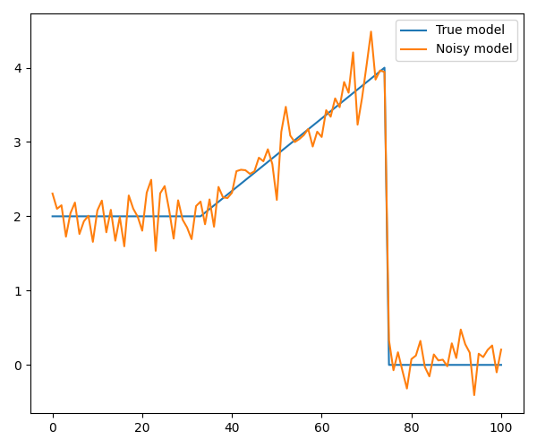
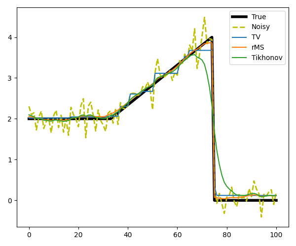
Next, we consider an example where we replace the first jump with a slope. As we will see, TV can not deal with this type of structure since a linear increase will greatly increase the TV norm, and instead TV will make a staircase. rMS, on the other hand, can reconstruct the model with high accuracy.

nx = 101
idx_jump1 = nx // 3
idx_jump2 = 3 * nx // 4
x = np.zeros(nx)
x[:idx_jump1] = 2
x[idx_jump1:idx_jump2] = np.linspace(2, 4, idx_jump2 - idx_jump1)
n = np.random.normal(0, 0.25, nx)
y = x + n

# Plot the model and the noisy data
fig, axs = plt.subplots(1, 1, figsize=(6, 5))
axs.plot(x, label='True model')
axs.plot(y, label='Noisy model')
axs.legend()
plt.tight_layout()

# Define functionals
l2 = pyproximal.proximal.L2(b=y)
l1 = pyproximal.proximal.L1(sigma=1.)
Dop = pylops.FirstDerivative(nx, edge=True, kind='backward')

# TV
L = np.real((Dop.H * Dop).eigs(neigs=1, which='LM')[0])
tau = 1.
mu = 0.99 * tau / L
xTV, _ = pyproximal.optimization.primal.LinearizedADMM(l2, l1, Dop, tau=tau, mu=mu,
                                                       x0=np.zeros_like(x), niter=200)

# rMS
sigma = 1e1
kappa = 1e0
ms_relaxed = pyproximal.proximal.RelaxedMumfordShah(sigma=sigma, kappa=kappa)
tau = 1.
mu = tau / L
xrMS, _ = pyproximal.optimization.primal.LinearizedADMM(l2, ms_relaxed, Dop, tau=tau, mu=mu,
                                                        x0=np.zeros_like(x), niter=200)

# Tikhonov
Op = pylops.Identity(nx)
Regs = [Dop, ]
epsR = [3e0, ]

xTikhonov = pylops.optimization.leastsquares.regularized_inversion(Op=Op, Regs=Regs, y=y, epsRs=epsR)[0]

# Plot the results
fig, axs = plt.subplots(1, 1, figsize=(6, 5))
axs.plot(x, label='True', linewidth=4, color='k')
axs.plot(y, '--', label='Noisy', linewidth=2, color='y')
axs.plot(xTV, label='TV')
axs.plot(xrMS, label='rMS')
axs.plot(xTikhonov, label='Tikhonov')
axs.legend()
plt.tight_layout()

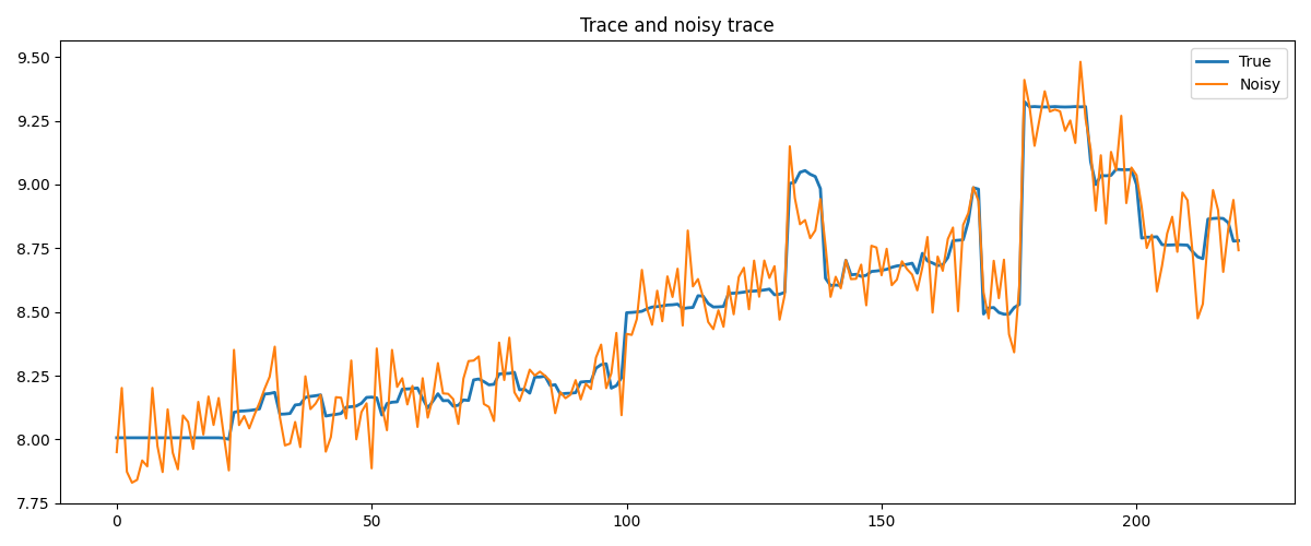
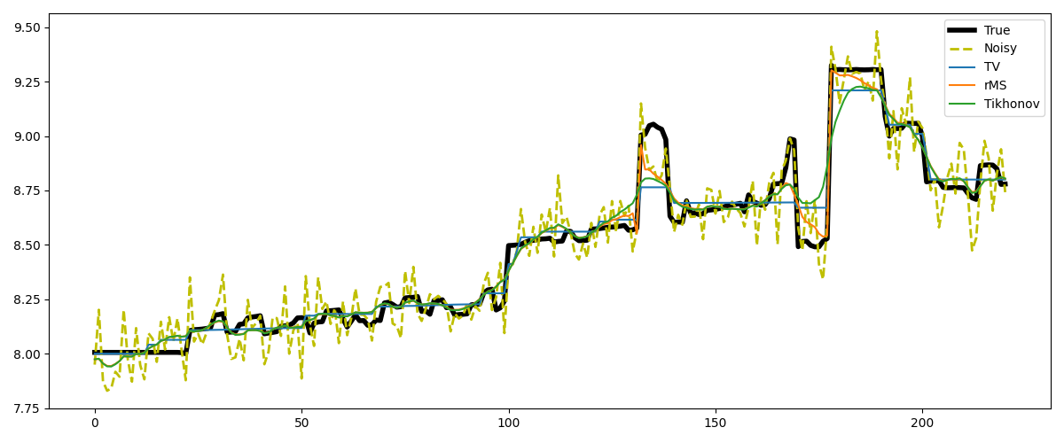
Finally, we take a trace from a section of the Marmousi model. This trace shows rather smooth behavior with a few jumps, which makes it perfectly suited for rMS. TV on the other hand will artificially create a staircasing effect.

# Get a trace from the model and add some noise
m_trace = np.load('../testdata/marmousi_trace.npy')
nz = len(m_trace)
m_trace_noisy = m_trace + np.random.normal(0, 0.1, nz)

# Plot the model and the noisy data
fig, ax = plt.subplots(1, 1, figsize=(12, 5))
ax.plot(m_trace, linewidth=2, label='True')
ax.plot(m_trace_noisy, label='Noisy')
ax.set_title('Trace and noisy trace')
ax.axis('tight')
ax.legend()
plt.tight_layout()

# Define functionals
l2 = pyproximal.proximal.L2(b=m_trace_noisy)
l1 = pyproximal.proximal.L1(sigma=5e-1)
Dop = pylops.FirstDerivative(nz, edge=True, kind='backward')

# TV
L = np.real((Dop.H * Dop).eigs(neigs=1, which='LM')[0])
tau = 1.
mu = 0.99 * tau / L
xTV, _ = pyproximal.optimization.primal.LinearizedADMM(l2, l1, Dop, tau=tau, mu=mu,
                                                       x0=np.zeros_like(m_trace), niter=200)

# rMS
sigma = 5e0
kappa = 1e-1
ms_relaxed = pyproximal.proximal.RelaxedMumfordShah(sigma=sigma, kappa=kappa)

tau = 1.
mu = tau / L
xrMS, _ = pyproximal.optimization.primal.LinearizedADMM(l2, ms_relaxed, Dop, tau=tau, mu=mu,
                                                        x0=np.zeros_like(m_trace), niter=200)

# Tikhonov
Op = pylops.Identity(nz)
Regs = [Dop, ]
epsR = [3e0, ]

xTikhonov = pylops.optimization.leastsquares.regularized_inversion(Op=Op, Regs=Regs,
                                                                   y=m_trace_noisy,
                                                                   epsRs=epsR)[0]

# Plot the results
fig, axs = plt.subplots(1, 1, figsize=(12, 5))
axs.plot(m_trace, label='True', linewidth=4, color='k')
axs.plot(m_trace_noisy, '--', label='Noisy', linewidth=2, color='y')
axs.plot(xTV, label='TV')
axs.plot(xrMS, label='rMS')
axs.plot(xTikhonov, label='Tikhonov')
axs.legend()
plt.tight_layout()