Hankel matrix estimation

A Hankel matrix is a matrix with constant anti-diagonals. Such matrices frequently occur in statistics and engineering applications, e.g. in the study of non-stationary signals and estimation of population parameters (method of moments).

In this tutorial, we will consider a linear dynamical system, cf. section 4.1 in 1. Here, the rank of the corresponding Hankel matrix is connected to the complexity of the system. More precisely, if a signal \(f\) is a linear combination of \(r_0\) complex exponentials (with arbitrary frequencies) then \(H(f)\) is of rank \(r_0\).

Given a noisy measurement matrix \(X_0\) we therefore seek to minimize:

\[\min_{X\in\mathcal{H},\,\rank(X)\leq r_0} \| X - X_0 \|_F\]

where \(\mathcal{H}\) is the set of Hankel matrices.

References

1

Larsson, V. and Olsson, C. “Convex Low Rank Approximation”, In International Journal of Computer Vision (IJCV), 120:194–214, 2016.

import matplotlib.pyplot as plt
import numpy as np
from scipy.linalg import hankel

from pyproximal.optimization.primal import ADMM
from pyproximal.projection import HankelProj
from pyproximal.proximal import Hankel, QuadraticEnvelopeRankL2


plt.close('all')
np.random.seed(0)

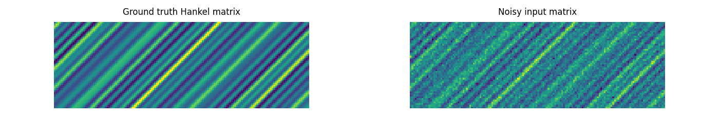
We generate a Hankel matrix by randomly sampling a sinusoidal signal

\[f(t) = \sum_{i=1}^N e^{d_i(t-t_i)}\cos(\phi_i(t-t_i)),\]

where \(d_i\), \(\phi_i\) and \(t_i\) are sampled from a uniform distribution.

n_signal = 5
t = np.linspace(-1, 1, 200)
f_gt = np.zeros_like(t)

for i in range(n_signal):
    d = np.random.uniform(-1, 1)
    phi = np.random.uniform(-40 * np.pi, 40 * np.pi)
    t0 = np.random.uniform(-1, 1)
    f_gt += np.exp(d * (t - t0)) * np.cos(phi * (t - t0))

Note that the rank of the corresponding Hankel matrix is twice the number of sinusoidals, since each term can be expressed by two complex exponentials.

r0 = 2 * n_signal

# Create the corresponding Hankel matrix
X_gt = hankel(f_gt[:51], f_gt[50:])

# Add noise
sigma = 1
X0 = X_gt + np.random.normal(0, sigma, X_gt.shape)

Now we compare the ground truth with the noisy input data

fig, axs = plt.subplots(1, 2, figsize=(14, 7/3))
axs[0].imshow(X_gt)
axs[0].set_title('Ground truth Hankel matrix')
axs[0].axis('equal')
axs[0].axis('off')
axs[1].imshow(X0)
axs[1].set_title('Noisy input matrix')
axs[1].axis('equal')
axs[1].axis('off')
plt.tight_layout()

Relaxation 1: Enforcing the Hankel matrix constraint only

Let us take one step back and consider the original problem formulation. Solving it directly is not straight-forward, since it is non-convex and the rank constraint introduces discontinuities. Thus, one is forced to consider relaxations of the original problem formulation, e.g. one could ignore the rank constraint, i.e.

\[\min_{X\in\mathcal{H}} \| X - X_0 \|_F \; .\]

This is simply the projection onto the set of Hankel matrices.

hankel_proj = HankelProj()
X_rec_hankel = hankel_proj(X0)

Relaxation 2: Low-rank approximation

Instead, we can discard the Hankel matrix constraint and consider the low rank approximation problem

\[\min_{\rank(X)\leq r_0} \| X - X_0 \|_F\]

which has a closed form solution (by the Eckart–Young theorem).

U, S, Vh = np.linalg.svd(X0, full_matrices=False)
X_rec_lowrank = (U[:, :r0] * S[:r0]) @ Vh[:r0, :]

Relaxation 3: Quadratic envelope relaxation of the rank constraint

Let us now try to improve the results and come closer to the cost function originally proposed. This can be done by relaxing the rank constraint with the quadratic envelope of the rank function \(\mathcal{R}_{r_0}\). We therefore consider minimizing the cost function

\[\min_{X\in\mathcal{H}} \mathcal{R}_{r_0}(X) + \frac{1}{2}\| X - X_0 \|_F^2\]

One way to solve such problems is to utilize splitting schemes. For this tutorial, we chose to work with pyproximal.ADMM. In order to do so, we introduce a new variable \(Z\) and consider the equivalent formulation

\[\min_{X,\,Z} \mathcal{R}_{r_0}(X) + \frac{1}{2}\| X - X_0 \|_F^2 + \mathcal{I}_{\mathcal{H}}(Z)\]

where \(\mathcal{I}_{\mathcal{H}}\) is the indicator function for the set of Hankel matrices. Furthermore, we must add the constraint \(X = Z\).

The \(Z\) update is simply a projection onto the set of Hankel matrices, but the \(X\) update requires solving

\[\argmin_{X} \mathcal{R}_{r_0}(X) + \frac{1}{2}\| X - X_0 \|_F^2 + \frac{1}{2\tau}\| X - U \|_F^2\]

which is implemented in pyproximal.QuadraticEnvelopeRankL2.

proxf = QuadraticEnvelopeRankL2(X0.shape, r0, X0)
proxg = Hankel(X0.shape)
X_rec_quadenv = ADMM(proxf, proxg, x0=X0.ravel(), tau=0.5, niter=200)[0]
X_rec_quadenv = X_rec_quadenv.reshape(X0.shape)

Let us compare the results

fig, axs = plt.subplots(1, 3, figsize=(21, 7/3))
axs[0].imshow(X_rec_hankel)
axs[0].set_title('Recovery by projection onto set of Hankel matrices')
axs[0].axis('equal')
axs[0].axis('off')
axs[0].axis('tight')
axs[1].imshow(X_rec_lowrank)
axs[1].set_title('Recovery by low-rank approximation')
axs[1].axis('equal')
axs[1].axis('off')
axs[1].axis('tight')
axs[2].imshow(X_rec_quadenv)
axs[2].set_title('Recovery by quadratic envelope relaxation')
axs[2].axis('off')
axs[2].axis('equal')
axs[2].axis('tight')
plt.tight_layout()

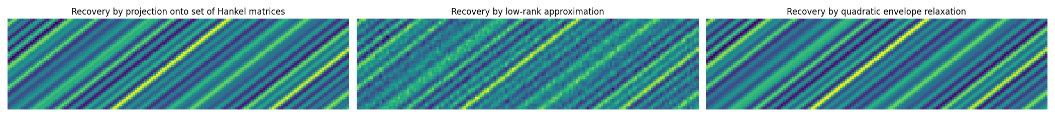
It can be hard to compare by ocular inspection, so let us measure the actual numbers. First, we consider the Frobenius norm error for the different reconstructions

metric = lambda X: np.linalg.norm(X_gt - X, "fro")
print(f'Projection onto set of Hankel matrices:')
print(f'Rec. error: {metric(X_rec_hankel):.4f}')
print(f'Low-rank approximation:')
print(f'Rec. error: {metric(X_rec_lowrank):.4f}')
print(f'Quadratic envelope relaxation:')
print(f'Rec. error: {metric(X_rec_quadenv):.4f}')

Projection onto set of Hankel matrices:
Rec. error: 13.8851
Low-rank approximation:
Rec. error: 44.8668
Quadratic envelope relaxation:
Rec. error: 4.9923

Of course, we also know the sought rank, which gives us another useful metric, namely the sum of the smallest singular values (which ought to vanish if the reconstruction is correct)

metric = lambda X: np.sum(np.linalg.svd(X, compute_uv=False)[r0:])
print(f'Projection onto set of Hankel matrices:')
print(f'Sum of sing. val. > r0: {metric(X_rec_hankel):.4f}')
print(f'Low-rank approximation:')
print(f'Sum of sing. val. > r0: {metric(X_rec_lowrank):.4e}')
print(f'Quadratic envelope relaxation:')
print(f'Sum of sing. val. > r0: {metric(X_rec_quadenv):.4e}')

Projection onto set of Hankel matrices:
Sum of sing. val. > r0: 74.4629
Low-rank approximation:
Sum of sing. val. > r0: 1.8417e-13
Quadratic envelope relaxation:
Sum of sing. val. > r0: 6.8227e-13

In conclusion, by enforcing both constraints actively, i.e. the Hankel matrix constraint and the rank constraint, we get an improved overall result while preserving the known rank.