Note
Go to the end to download the full example code.
Group sparsity
This notebooks considers the problem of jointly interpolating N (e.g., 2) signals
with sparse representation in the frequency domain and shows the importance of applying
a group sparsity constraint by means of the pyproximal.proximal.L01Ball proximal operator.
Given the following problem:
we aim to find a solution to this objective function:
where \(\mathbf{X}\) is a matrix whose rows are represented by the different signals \(\mathbf{x}_i\), and the \(L_{0,1}\) norm computes the number of non-zero elements of a vector whose elements are the $L_1$ norm of each column of \(\mathbf{X}\).
import matplotlib.pyplot as plt
import numpy as np
import pylops

import pyproximal

plt.close("all")
np.random.seed(10)
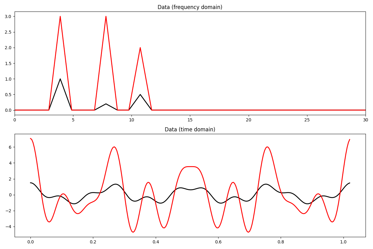
Let’s first create 2 signals in the frequency domain composed by the superposition of 3 sinusoids with different frequencies.
ifreqs = [4, 8, 11]
amps1 = [1.0, 0.2, 0.5]
amps2 = [3.0, 3.0, 2.0]

N = 2**8
nfft = N
dt = 0.004
t = np.arange(N) * dt
f = np.fft.rfftfreq(nfft, dt)

FFTop = 10 * pylops.signalprocessing.FFT(N, nfft=nfft, real=True)

X1 = np.zeros(nfft // 2 + 1, dtype="complex128")
X2 = np.zeros(nfft // 2 + 1, dtype="complex128")
X1[ifreqs] = amps1
X2[ifreqs] = amps2

x1 = FFTop.H * X1
x2 = FFTop.H * X2

fig, axs = plt.subplots(2, 1, figsize=(12, 8))
axs[0].plot(f, np.abs(X1), "k", lw=2)
axs[0].plot(f, np.abs(X2), "r", lw=2)
axs[0].set_xlim(0, 30)
axs[0].set_title("Data (frequency domain)")
axs[1].plot(t, x1, "k", lw=2)
axs[1].plot(t, x2, "r", lw=2)
axs[1].set_title("Data (time domain)")
axs[1].axis("tight")
plt.tight_layout()
We now define the locations at which the signals will be sampled. The first signal is severely subsampled (10% of available samples), whilst the second dataset retains 60% of its samples. This choice is made on purpose to see if group sparsity could help interpolating the first signal by leveraging the fact that it is easier to interpolate the second signal
np.random.seed(10)

perc_subsampling = (0.1, 0.6)
Nsub1, Nsub2 = (
    int(np.round(N * perc_subsampling[0])),
    int(np.round(N * perc_subsampling[1])),
)
iava1 = np.sort(np.random.permutation(np.arange(N))[:Nsub1])
iava2 = np.sort(np.random.permutation(np.arange(N))[:Nsub2])

# Create restriction operator
Rop1 = pylops.Restriction(N, iava1, dtype="float64")
Rop2 = pylops.Restriction(N, iava2, dtype="float64")

y1 = Rop1 * x1
y2 = Rop2 * x2

Op1 = Rop1 * FFTop.H
Op2 = Rop2 * FFTop.H

X1adj = Op1.H * y1
X2adj = Op2.H * y2
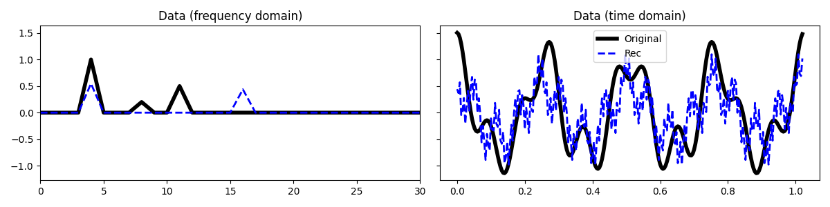
Let’s try to interpolate the first signal
L = np.abs((Op1.H * Op1).eigs(1)[0])
eps = 1  # not used given that a projection is used as regularizer
niter = 400
tau = 0.95 / L

l0 = pyproximal.proximal.L0Ball(3)
l2 = pyproximal.proximal.L2(Op=Op1, b=y1)
X1est = pyproximal.optimization.primal.ProximalGradient(
    l2,
    l0,
    tau=tau,
    x0=np.zeros(nfft // 2 + 1, dtype="complex128"),
    epsg=eps,
    niter=niter,
    acceleration="fista",
    show=False,
)
x1est = FFTop.H * X1est

fig, axs = plt.subplots(1, 2, sharey=True, figsize=(12, 3))
axs[0].plot(np.abs(X1), "k", lw=4, label="Original")
axs[0].plot(np.abs(X1est), "--b", lw=2, label="Rec")
axs[0].set_title("Data (frequency domain)")
axs[0].set_xlim(0, 30)
axs[1].plot(t, x1, "k", lw=4, label="Original")
axs[1].plot(t, x1est, "--b", lw=2, label="Rec")
axs[1].set_title("Data (time domain)")
axs[1].legend()
plt.tight_layout()
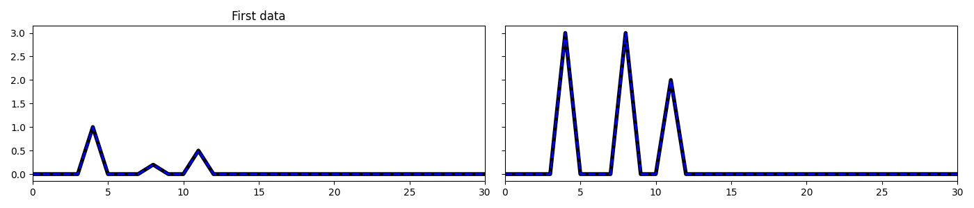
And now we interpolate the two signals together
Opp = pylops.BlockDiag([Op1, Op2])
yy = np.hstack([y1, y2])

L = np.abs((Opp.H * Opp).eigs(1)[0])
eps = 1  # not used given that a projection is used as regularizer
niter = 400
tau = 0.99 / L

l0 = pyproximal.proximal.L10Ball(ndim=2, radius=4)
l2 = pyproximal.proximal.L2(Op=Opp, b=yy)

XXest = pyproximal.optimization.primal.ProximalGradient(
    l2,
    l0,
    tau=tau,
    x0=np.zeros(2 * (nfft // 2 + 1), dtype="complex128"),
    epsg=eps,
    niter=niter,
    acceleration="fista",
    show=False,
)

X1est, X2est = XXest[: FFTop.shape[0]], XXest[FFTop.shape[0] :]
x1est = FFTop.H * X1est
x2est = FFTop.H * X2est
/home/docs/checkouts/readthedocs.org/user_builds/pyproximal/envs/latest/lib/python3.13/site-packages/numpy/lib/_shape_base_impl.py:274: ComplexWarning: Casting complex values to real discards the imaginary part
  arr[_make_along_axis_idx(arr_shape, indices, axis)] = values
We can see that the first signal is now much better interpolated
fig, axs = plt.subplots(1, 2, sharey=True, figsize=(14, 3))
axs[0].plot(np.abs(X1), "k", lw=4, label="Original")
axs[0].plot(np.abs(X1est), "--b", lw=2, label="Rec")
axs[0].set_title("First data")
axs[1].plot(np.abs(X2), "k", lw=4)
axs[1].plot(np.abs(X2est), "--b", lw=2)
axs[0].set_xlim(0, 30)
axs[1].set_xlim(0, 30)
plt.tight_layout()
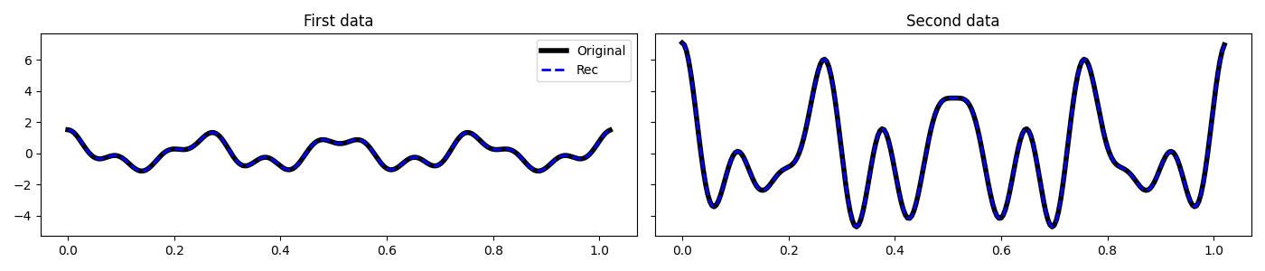
And similarly the second signal is also better interpolated
fig, axs = plt.subplots(1, 2, sharey=True, figsize=(14, 3))
axs[0].plot(t, x1, "k", lw=4, label="Original")
axs[0].plot(t, x1est, "--b", lw=2, label="Rec")
axs[0].set_title("First data")
axs[0].legend()
axs[1].plot(t, x2, "k", lw=4)
axs[1].plot(t, x2est, "--b", lw=2)
axs[1].set_title("Second data")
plt.tight_layout()
Total running time of the script: (0 minutes 1.025 seconds)