Note
Go to the end to download the full example code.
Denoising
This tutorial considers the classical problem of denoising of images affected by either random noise or salt-and-pepper noise using proximal algorithms.
The overall cost function to minimize is written in the following form:
where the L2 norm in the data term can be replaced by a L1 norm for salt-and-pepper (outlier like noise).
For both examples we investigate with different choices of regularization:
L2 on Gradient \(J(\mathbf{u}) = \|\nabla \mathbf{u}\|_2^2\)
Anisotropic TV \(J(\mathbf{u}) = \|\nabla \mathbf{u}\|_1\)
Isotropic TV \(J(\mathbf{u}) = \|\nabla \mathbf{u}\|_{2,1}\)
import matplotlib.pyplot as plt
import numpy as np
import pylops
from scipy import datasets

import pyproximal

plt.close("all")
np.random.seed(10)
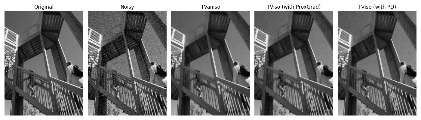
Let’s start by loading a sample image and adding some noise
We can now define a pylops.Gradient operator that we are going to
use for all regularizers
We then consider the first regularization (L2 norm on Gradient). We expect to get a smooth image where noise is suppressed by sharp edges in the original image are however lost.
# L2 data term
l2 = pyproximal.L2(b=noise_img.ravel())

# L2 regularization
sigma = 2.0
thik = pyproximal.L2(sigma=sigma)

# Solve
tau = 1.0
mu = 1.0 / (tau * L)

iml2 = pyproximal.optimization.primal.LinearizedADMM(
    l2, thik, Gop, tau=tau, mu=mu, x0=np.zeros_like(img.ravel()), niter=100
)[0]
iml2 = iml2.reshape(img.shape)
Let’s try now to use TV regularization, both anisotropic and isotropic
# L2 data term
l2 = pyproximal.L2(b=noise_img.ravel())

# Anisotropic TV
sigma = 0.1
l1 = pyproximal.L1(sigma=sigma)

# Solve
tau = 1.0
mu = tau / L

iml1 = pyproximal.optimization.primal.LinearizedADMM(
    l2, l1, Gop, tau=tau, mu=mu, x0=np.zeros_like(img.ravel()), niter=100
)[0]
iml1 = iml1.reshape(img.shape)


# Isotropic TV with Proximal Gradient
sigma = 0.1
tv = pyproximal.TV(dims=img.shape, sigma=sigma)

# Solve
tau = 1 / L

imtv = pyproximal.optimization.primal.ProximalGradient(
    l2, tv, tau=tau, x0=np.zeros_like(img.ravel()), niter=100
)
imtv = imtv.reshape(img.shape)

# Isotropic TV with Primal Dual
sigma = 0.1
l1iso = pyproximal.L21(ndim=2, sigma=sigma)

# Solve
tau = 1 / np.sqrt(L)
mu = 1.0 / (tau * L)

iml12 = pyproximal.optimization.primaldual.PrimalDual(
    l2, l1iso, Gop, tau=tau, mu=mu, theta=1.0, x0=np.zeros_like(img.ravel()), niter=100
)
iml12 = iml12.reshape(img.shape)

fig, axs = plt.subplots(1, 5, figsize=(14, 4))
axs[0].imshow(img, cmap="gray", vmin=0, vmax=1)
axs[0].set_title("Original")
axs[0].axis("off")
axs[0].axis("tight")
axs[1].imshow(noise_img, cmap="gray", vmin=0, vmax=1)
axs[1].set_title("Noisy")
axs[1].axis("off")
axs[1].axis("tight")
axs[2].imshow(iml1, cmap="gray", vmin=0, vmax=1)
axs[2].set_title("TVaniso")
axs[2].axis("off")
axs[2].axis("tight")
axs[3].imshow(imtv, cmap="gray", vmin=0, vmax=1)
axs[3].set_title("TViso (with ProxGrad)")
axs[3].axis("off")
axs[3].axis("tight")
axs[4].imshow(iml12, cmap="gray", vmin=0, vmax=1)
axs[4].set_title("TViso (with PD)")
axs[4].axis("off")
axs[4].axis("tight")
plt.tight_layout()
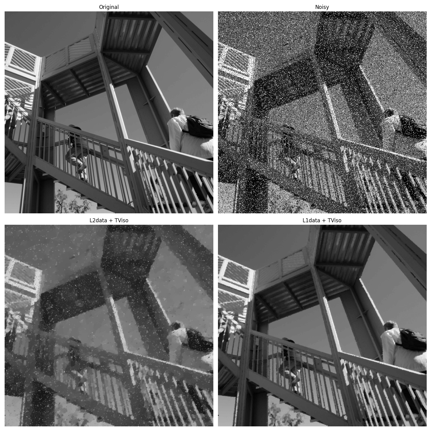
Finally we consider an example where the original image is corrupted by salt-and-pepper noise.
# Add salt and pepper noise
noiseperc = 0.1

isalt = np.random.permutation(np.arange(ny * nx))[: int(noiseperc * ny * nx)]
ipepper = np.random.permutation(np.arange(ny * nx))[: int(noiseperc * ny * nx)]
noise_img = img.copy().ravel()
noise_img[isalt] = img.max()
noise_img[ipepper] = img.min()
noise_img = noise_img.reshape(ny, nx)
Here we compare L2 and L1 norms for the data term L2 data term
l2 = pyproximal.L2(b=noise_img.ravel())

# L1 regularization (isotropic TV)
sigma = 0.2
l1iso = pyproximal.L21(ndim=2, sigma=sigma)

# Solve
tau = 0.1
mu = 1.0 / (tau * L)

iml12_l2 = pyproximal.optimization.primaldual.PrimalDual(
    l2,
    l1iso,
    Gop,
    tau=tau,
    mu=mu,
    theta=1.0,
    x0=np.zeros_like(noise_img).ravel(),
    niter=100,
    show=True,
)
iml12_l2 = iml12_l2.reshape(img.shape)


# L1 data term
l1 = pyproximal.L1(g=noise_img.ravel())

# L1 regularization (isotropic TV)
sigma = 0.7
l1iso = pyproximal.L21(ndim=2, sigma=sigma)

# Solve
tau = 1.0
mu = 1.0 / (tau * L)

iml12_l1 = pyproximal.optimization.primaldual.PrimalDual(
    l1,
    l1iso,
    Gop,
    tau=tau,
    mu=mu,
    theta=1.0,
    x0=np.zeros_like(noise_img).ravel(),
    niter=100,
    show=True,
)
iml12_l1 = iml12_l1.reshape(img.shape)

fig, axs = plt.subplots(2, 2, figsize=(14, 14))
axs[0][0].imshow(img, cmap="gray", vmin=0, vmax=1)
axs[0][0].set_title("Original")
axs[0][0].axis("off")
axs[0][0].axis("tight")
axs[0][1].imshow(noise_img, cmap="gray", vmin=0, vmax=1)
axs[0][1].set_title("Noisy")
axs[0][1].axis("off")
axs[0][1].axis("tight")
axs[1][0].imshow(iml12_l2, cmap="gray", vmin=0, vmax=1)
axs[1][0].set_title("L2data + TViso")
axs[1][0].axis("off")
axs[1][0].axis("tight")
axs[1][1].imshow(iml12_l1, cmap="gray", vmin=0, vmax=1)
axs[1][1].set_title("L1data + TViso")
axs[1][1].axis("off")
axs[1][1].axis("tight")
plt.tight_layout()
PrimalDual
-------------------------------------------------------------------------------------
Proximal operator (f): L2
Proximal operator (g): L21
Linear operator (A): Gradient
Additional vector (z): None

tau = 0.1       mu = 1.25       theta = 1.00e+00
tol = None      niter = 100
-------------------------------------------------------------------------------------

    Itn           x[0]                 f            g          z^x       J=f+g+z^x
     1         2.9590e-02          2.3279e+04  1.4716e+03   0.0000e+00   2.4750e+04
     2         5.6409e-02          2.0204e+04  1.6498e+03   0.0000e+00   2.1854e+04
     3         8.0676e-02          1.7777e+04  1.6009e+03   0.0000e+00   1.9378e+04
     4         1.0058e-01          1.5785e+04  1.5497e+03   0.0000e+00   1.7335e+04
     5         1.1584e-01          1.4131e+04  1.5324e+03   0.0000e+00   1.5664e+04
     6         1.2779e-01          1.2751e+04  1.5358e+03   0.0000e+00   1.4287e+04
     7         1.3807e-01          1.1598e+04  1.5500e+03   0.0000e+00   1.3148e+04
     8         1.4774e-01          1.0634e+04  1.5711e+03   0.0000e+00   1.2205e+04
     9         1.5714e-01          9.8294e+03  1.5963e+03   0.0000e+00   1.1426e+04
    10         1.6613e-01          9.1585e+03  1.6231e+03   0.0000e+00   1.0782e+04
    11         1.7448e-01          8.5996e+03  1.6494e+03   0.0000e+00   1.0249e+04
    21         2.3789e-01          6.2461e+03  1.8205e+03   0.0000e+00   8.0666e+03
    31         2.8852e-01          5.8395e+03  1.8871e+03   0.0000e+00   7.7267e+03
    41         2.9634e-01          5.7576e+03  1.9117e+03   0.0000e+00   7.6693e+03
    51         3.0009e-01          5.7372e+03  1.9201e+03   0.0000e+00   7.6573e+03
    61         3.0252e-01          5.7310e+03  1.9226e+03   0.0000e+00   7.6537e+03
    71         3.0289e-01          5.7289e+03  1.9231e+03   0.0000e+00   7.6520e+03
    81         3.0341e-01          5.7281e+03  1.9230e+03   0.0000e+00   7.6511e+03
    91         3.0361e-01          5.7279e+03  1.9227e+03   0.0000e+00   7.6505e+03
    92         3.0361e-01          5.7278e+03  1.9226e+03   0.0000e+00   7.6505e+03
    93         3.0361e-01          5.7278e+03  1.9226e+03   0.0000e+00   7.6504e+03
    94         3.0360e-01          5.7278e+03  1.9226e+03   0.0000e+00   7.6504e+03
    95         3.0360e-01          5.7278e+03  1.9225e+03   0.0000e+00   7.6503e+03
    96         3.0359e-01          5.7278e+03  1.9225e+03   0.0000e+00   7.6503e+03
    97         3.0358e-01          5.7278e+03  1.9224e+03   0.0000e+00   7.6502e+03
    98         3.0357e-01          5.7278e+03  1.9224e+03   0.0000e+00   7.6502e+03
    99         3.0356e-01          5.7278e+03  1.9224e+03   0.0000e+00   7.6502e+03
   100         3.0356e-01          5.7278e+03  1.9223e+03   0.0000e+00   7.6501e+03

Iterations = 100        Total time (s) = 1.45
-------------------------------------------------------------------------------------

PrimalDual
-------------------------------------------------------------------------------------
Proximal operator (f): L1
Proximal operator (g): L21
Linear operator (A): Gradient
Additional vector (z): None

tau = 1.0       mu = 0.125      theta = 1.00e+00
tol = None      niter = 100
-------------------------------------------------------------------------------------

    Itn           x[0]                 f            g          z^x       J=f+g+z^x
     1         3.2549e-01          0.0000e+00  5.6656e+04   0.0000e+00   5.6656e+04
     2         3.2549e-01          0.0000e+00  5.6656e+04   0.0000e+00   5.6656e+04
     3         3.2549e-01          2.3690e+03  5.1165e+04   0.0000e+00   5.3534e+04
     4         3.2549e-01          9.0647e+03  3.6533e+04   0.0000e+00   4.5598e+04
     5         3.2549e-01          1.6544e+04  2.6898e+04   0.0000e+00   4.3442e+04
     6         3.2549e-01          2.1677e+04  2.3751e+04   0.0000e+00   4.5428e+04
     7         3.2549e-01          2.3954e+04  2.1118e+04   0.0000e+00   4.5071e+04
     8         3.2549e-01          2.4367e+04  1.7295e+04   0.0000e+00   4.1662e+04
     9         3.2549e-01          2.4089e+04  1.4659e+04   0.0000e+00   3.8748e+04
    10         3.2549e-01          2.3807e+04  1.3194e+04   0.0000e+00   3.7001e+04
    11         3.2549e-01          2.3746e+04  1.2090e+04   0.0000e+00   3.5836e+04
    21         3.2549e-01          2.4769e+04  7.5068e+03   0.0000e+00   3.2276e+04
    31         3.2549e-01          2.4918e+04  6.8042e+03   0.0000e+00   3.1722e+04
    41         3.2549e-01          2.4968e+04  6.5645e+03   0.0000e+00   3.1533e+04
    51         3.2549e-01          2.4991e+04  6.4324e+03   0.0000e+00   3.1423e+04
    61         3.2549e-01          2.5012e+04  6.3361e+03   0.0000e+00   3.1348e+04
    71         3.2549e-01          2.5025e+04  6.2663e+03   0.0000e+00   3.1292e+04
    81         3.2549e-01          2.5032e+04  6.2178e+03   0.0000e+00   3.1249e+04
    91         3.2549e-01          2.5040e+04  6.1723e+03   0.0000e+00   3.1213e+04
    92         3.2549e-01          2.5042e+04  6.1678e+03   0.0000e+00   3.1210e+04
    93         3.2549e-01          2.5044e+04  6.1630e+03   0.0000e+00   3.1207e+04
    94         3.2549e-01          2.5046e+04  6.1577e+03   0.0000e+00   3.1204e+04
    95         3.2549e-01          2.5048e+04  6.1531e+03   0.0000e+00   3.1201e+04
    96         3.2549e-01          2.5049e+04  6.1494e+03   0.0000e+00   3.1199e+04
    97         3.2549e-01          2.5050e+04  6.1457e+03   0.0000e+00   3.1196e+04
    98         3.2549e-01          2.5052e+04  6.1408e+03   0.0000e+00   3.1192e+04
    99         3.2549e-01          2.5053e+04  6.1370e+03   0.0000e+00   3.1190e+04
   100         3.2549e-01          2.5054e+04  6.1340e+03   0.0000e+00   3.1188e+04

Iterations = 100        Total time (s) = 1.51
-------------------------------------------------------------------------------------
Total running time of the script: (0 minutes 23.289 seconds)