Note
Go to the end to download the full example code.
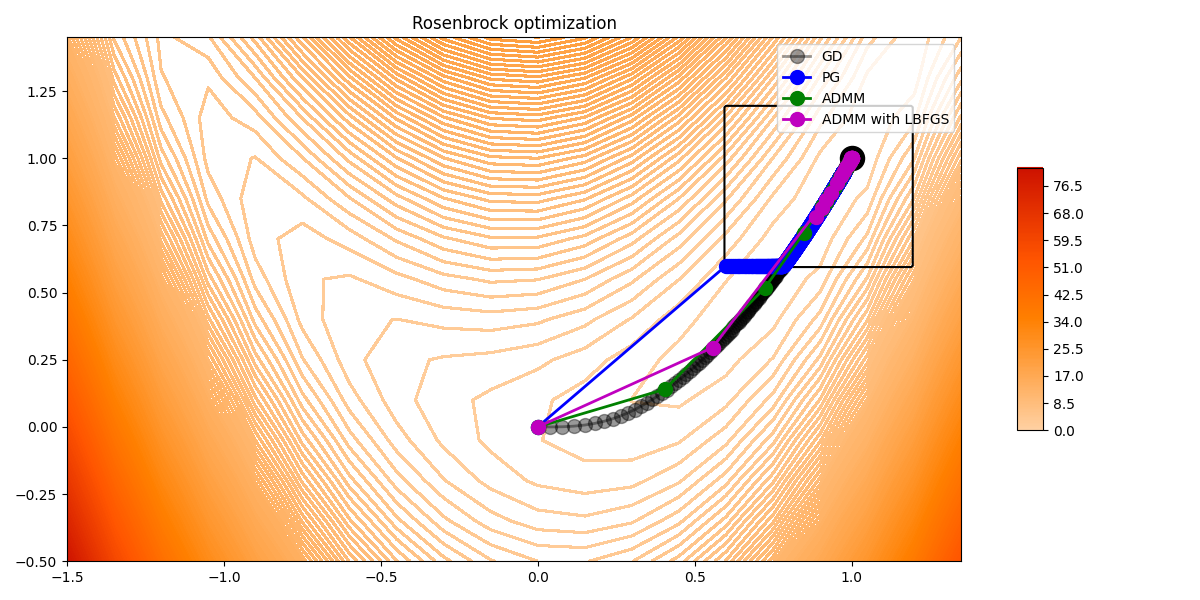
Nonlinear inversion with box constraints
In this tutorial we focus on a modification of the Quadratic program with box constraints tutorial where the quadratic function is replaced by a nonlinear function:
For this example we will use the well-known Rosenbrock function:
where \(\mathbf{x}=[x, y]\), \(a=1\), and \(b=10\).
We will learn how to handle nonlinear functionals in convex optimization, and
more specifically dive into the details of the
pyproximal.proximal.Nonlinear operator. This is a template operator
which must be subclassed and used for a specific functional. After doing so, we will
need to implement the following three method: func and grad and optimize.
As the names imply, the first method takes a model vector \(x\) as input and
evaluates the functional. The second method evaluates the gradient of the
functional with respect to \(x\). The third method implements an
optimization routine that solves the proximal operator of \(f\),
more specifically:
Note that when creating the optimize method a user must use the gradient
of the augmented functional which is provided by the _gradprox built-in
method in pyproximal.proximal.Nonlinear class.
In this example, we will consider both the
pyproximal.optimization.primal.ProximalGradient and
pyproximal.optimization.primal.ADMM algorithms. The former solver
will simply use the grad method whilst the second solver relies on the
optimize method.
import matplotlib.pyplot as plt
import numpy as np
import scipy as sp

import pyproximal

plt.close("all")
np.random.seed(10)
Let’s start by defining the class for the nonlinear functional
def callback(x, xhist):
    xhist.append(x)


def rosenbrock(x, y, a=1, b=10):
    f = (a - x) ** 2 + b * (y - x**2) ** 2
    return f


def rosenbrock_grad(x, y, a=1, b=10):
    dfx = -2 * (a - x) - 2 * b * (y - x**2) * 2 * x
    dfy = 2 * b * (y - x**2)
    return dfx, dfy


def contour_rosenbrock(x, y):
    fig, ax = plt.subplots(figsize=(12, 6))

    # Evaluate the function
    x, y = np.meshgrid(x, y)
    z = rosenbrock(x, y)

    # Plot the surface.
    surf = ax.contour(
        x, y, z, 200, cmap="gist_heat_r", vmin=-20, vmax=200, antialiased=False
    )
    fig.colorbar(surf, shrink=0.5, aspect=10)
    return fig, ax


class Rosebrock(pyproximal.proximal.Nonlinear):
    def setup(self, a=1, b=10, alpha=1.0):
        self.a, self.b = a, b
        self.alpha = alpha

    def fun(self, x):
        return np.array(rosenbrock(x[0], x[1], a=self.a, b=self.b))

    def grad(self, x):
        return np.array(rosenbrock_grad(x[0], x[1], a=self.a, b=self.b))

    def optimize(self):
        self.solhist = []
        sol = self.x0.copy()
        for _ in range(self.niter):
            x1, x2 = sol
            dfx1, dfx2 = self._gradprox(sol, self.tau)
            x1 -= self.alpha * dfx1
            x2 -= self.alpha * dfx2
            sol = np.array([x1, x2])
            self.solhist.append(sol)
        self.solhist = np.array(self.solhist)
        return sol
We can now setup the problem and solve it without constraints using a simple gradient descent with fixed-step size (of course we could choose any other solver)
Let’s now define the box constraint
xbound = np.arange(-1.5, 1.5, 0.01)
ybound = np.arange(-0.5, 1.5, 0.01)
X, Y = np.meshgrid(xbound, ybound, indexing="ij")
xygrid = np.vstack((X.ravel(), Y.ravel()))

lower = 0.6
upper = 1.2
indic = (xygrid > lower) & (xygrid < upper)
indic = indic[0].reshape(xbound.size, ybound.size) & indic[1].reshape(
    xbound.size, ybound.size
)
ind = pyproximal.proximal.Box(lower, upper)
We now solve the constrained optimization using the Proximal gradient solver
x0 = np.array([0, 0])
fnl = Rosebrock(niter=20, x0=x0)
fnl.setup(1, 10, alpha=0.02)

xhist = [
    x0,
]
xinv_pg = pyproximal.optimization.primal.ProximalGradient(
    fnl,
    ind,
    tau=0.001,
    x0=x0,
    epsg=1.0,
    niter=5000,
    show=True,
    itershow=(10, 500, 10),
    callback=lambda x: callback(x, xhist),
)
xhist_pg = np.array(xhist)
ProximalGradient
---------------------------------------------------------------------------------
Proximal operator (f): Rosebrock
Proximal operator (g): Box
tau = 1.00e-03 backtrack = False
beta = 0.5 epsg = 1.0 acceleration = None
niter = 5000 niterback = 100 tol = None
---------------------------------------------------------------------------------
Itn x[0] f g J=f+eps*g tau
1 6.0000e-01 7.360e-01 1.000e+00 1.736e+00 1.00e-03
2 6.0656e-01 6.934e-01 1.000e+00 1.693e+00 1.00e-03
3 6.1298e-01 6.527e-01 1.000e+00 1.653e+00 1.00e-03
4 6.1925e-01 6.138e-01 1.000e+00 1.614e+00 1.00e-03
5 6.2538e-01 5.768e-01 1.000e+00 1.577e+00 1.00e-03
6 6.3135e-01 5.415e-01 1.000e+00 1.542e+00 1.00e-03
7 6.3717e-01 5.080e-01 1.000e+00 1.508e+00 1.00e-03
8 6.4284e-01 4.763e-01 1.000e+00 1.476e+00 1.00e-03
9 6.4836e-01 4.463e-01 1.000e+00 1.446e+00 1.00e-03
10 6.5372e-01 4.180e-01 1.000e+00 1.418e+00 1.00e-03
11 6.5893e-01 3.913e-01 1.000e+00 1.391e+00 1.00e-03
21 7.0268e-01 2.013e-01 1.000e+00 1.201e+00 1.00e-03
31 7.3281e-01 1.111e-01 1.000e+00 1.111e+00 1.00e-03
41 7.5245e-01 7.272e-02 1.000e+00 1.073e+00 1.00e-03
51 7.6476e-01 5.763e-02 1.000e+00 1.058e+00 1.00e-03
61 7.7230e-01 5.197e-02 1.000e+00 1.052e+00 1.00e-03
71 7.7684e-01 4.991e-02 1.000e+00 1.050e+00 1.00e-03
81 7.7970e-01 4.899e-02 1.000e+00 1.049e+00 1.00e-03
91 7.8172e-01 4.835e-02 1.000e+00 1.048e+00 1.00e-03
101 7.8332e-01 4.778e-02 1.000e+00 1.048e+00 1.00e-03
111 7.8472e-01 4.724e-02 1.000e+00 1.047e+00 1.00e-03
121 7.8602e-01 4.671e-02 1.000e+00 1.047e+00 1.00e-03
131 7.8726e-01 4.619e-02 1.000e+00 1.046e+00 1.00e-03
141 7.8847e-01 4.567e-02 1.000e+00 1.046e+00 1.00e-03
151 7.8966e-01 4.516e-02 1.000e+00 1.045e+00 1.00e-03
161 7.9084e-01 4.466e-02 1.000e+00 1.045e+00 1.00e-03
171 7.9200e-01 4.416e-02 1.000e+00 1.044e+00 1.00e-03
181 7.9316e-01 4.367e-02 1.000e+00 1.044e+00 1.00e-03
191 7.9431e-01 4.318e-02 1.000e+00 1.043e+00 1.00e-03
201 7.9544e-01 4.271e-02 1.000e+00 1.043e+00 1.00e-03
211 7.9657e-01 4.224e-02 1.000e+00 1.042e+00 1.00e-03
221 7.9769e-01 4.177e-02 1.000e+00 1.042e+00 1.00e-03
231 7.9881e-01 4.131e-02 1.000e+00 1.041e+00 1.00e-03
241 7.9991e-01 4.086e-02 1.000e+00 1.041e+00 1.00e-03
251 8.0101e-01 4.041e-02 1.000e+00 1.040e+00 1.00e-03
261 8.0209e-01 3.997e-02 1.000e+00 1.040e+00 1.00e-03
271 8.0317e-01 3.953e-02 1.000e+00 1.040e+00 1.00e-03
281 8.0424e-01 3.910e-02 1.000e+00 1.039e+00 1.00e-03
291 8.0531e-01 3.868e-02 1.000e+00 1.039e+00 1.00e-03
301 8.0636e-01 3.826e-02 1.000e+00 1.038e+00 1.00e-03
311 8.0741e-01 3.785e-02 1.000e+00 1.038e+00 1.00e-03
321 8.0845e-01 3.744e-02 1.000e+00 1.037e+00 1.00e-03
331 8.0949e-01 3.703e-02 1.000e+00 1.037e+00 1.00e-03
341 8.1051e-01 3.663e-02 1.000e+00 1.037e+00 1.00e-03
351 8.1153e-01 3.624e-02 1.000e+00 1.036e+00 1.00e-03
361 8.1254e-01 3.585e-02 1.000e+00 1.036e+00 1.00e-03
371 8.1355e-01 3.547e-02 1.000e+00 1.035e+00 1.00e-03
381 8.1454e-01 3.509e-02 1.000e+00 1.035e+00 1.00e-03
391 8.1553e-01 3.472e-02 1.000e+00 1.035e+00 1.00e-03
401 8.1651e-01 3.435e-02 1.000e+00 1.034e+00 1.00e-03
411 8.1749e-01 3.398e-02 1.000e+00 1.034e+00 1.00e-03
421 8.1846e-01 3.362e-02 1.000e+00 1.034e+00 1.00e-03
431 8.1942e-01 3.326e-02 1.000e+00 1.033e+00 1.00e-03
441 8.2038e-01 3.291e-02 1.000e+00 1.033e+00 1.00e-03
451 8.2133e-01 3.256e-02 1.000e+00 1.033e+00 1.00e-03
461 8.2227e-01 3.222e-02 1.000e+00 1.032e+00 1.00e-03
471 8.2321e-01 3.188e-02 1.000e+00 1.032e+00 1.00e-03
481 8.2413e-01 3.155e-02 1.000e+00 1.032e+00 1.00e-03
491 8.2506e-01 3.122e-02 1.000e+00 1.031e+00 1.00e-03
501 8.2597e-01 3.089e-02 1.000e+00 1.031e+00 1.00e-03
511 8.2689e-01 3.057e-02 1.000e+00 1.031e+00 1.00e-03
521 8.2779e-01 3.025e-02 1.000e+00 1.030e+00 1.00e-03
531 8.2869e-01 2.993e-02 1.000e+00 1.030e+00 1.00e-03
541 8.2958e-01 2.962e-02 1.000e+00 1.030e+00 1.00e-03
551 8.3047e-01 2.931e-02 1.000e+00 1.029e+00 1.00e-03
561 8.3135e-01 2.901e-02 1.000e+00 1.029e+00 1.00e-03
571 8.3222e-01 2.871e-02 1.000e+00 1.029e+00 1.00e-03
581 8.3309e-01 2.841e-02 1.000e+00 1.028e+00 1.00e-03
591 8.3395e-01 2.812e-02 1.000e+00 1.028e+00 1.00e-03
601 8.3481e-01 2.783e-02 1.000e+00 1.028e+00 1.00e-03
611 8.3566e-01 2.754e-02 1.000e+00 1.028e+00 1.00e-03
621 8.3651e-01 2.726e-02 1.000e+00 1.027e+00 1.00e-03
631 8.3735e-01 2.698e-02 1.000e+00 1.027e+00 1.00e-03
641 8.3818e-01 2.670e-02 1.000e+00 1.027e+00 1.00e-03
651 8.3901e-01 2.643e-02 1.000e+00 1.026e+00 1.00e-03
661 8.3983e-01 2.616e-02 1.000e+00 1.026e+00 1.00e-03
671 8.4065e-01 2.589e-02 1.000e+00 1.026e+00 1.00e-03
681 8.4147e-01 2.563e-02 1.000e+00 1.026e+00 1.00e-03
691 8.4227e-01 2.536e-02 1.000e+00 1.025e+00 1.00e-03
701 8.4308e-01 2.511e-02 1.000e+00 1.025e+00 1.00e-03
711 8.4387e-01 2.485e-02 1.000e+00 1.025e+00 1.00e-03
721 8.4467e-01 2.460e-02 1.000e+00 1.025e+00 1.00e-03
731 8.4545e-01 2.435e-02 1.000e+00 1.024e+00 1.00e-03
741 8.4623e-01 2.410e-02 1.000e+00 1.024e+00 1.00e-03
751 8.4701e-01 2.386e-02 1.000e+00 1.024e+00 1.00e-03
761 8.4778e-01 2.362e-02 1.000e+00 1.024e+00 1.00e-03
771 8.4855e-01 2.338e-02 1.000e+00 1.023e+00 1.00e-03
781 8.4931e-01 2.315e-02 1.000e+00 1.023e+00 1.00e-03
791 8.5007e-01 2.291e-02 1.000e+00 1.023e+00 1.00e-03
801 8.5082e-01 2.268e-02 1.000e+00 1.023e+00 1.00e-03
811 8.5157e-01 2.246e-02 1.000e+00 1.022e+00 1.00e-03
821 8.5231e-01 2.223e-02 1.000e+00 1.022e+00 1.00e-03
831 8.5305e-01 2.201e-02 1.000e+00 1.022e+00 1.00e-03
841 8.5379e-01 2.179e-02 1.000e+00 1.022e+00 1.00e-03
851 8.5452e-01 2.157e-02 1.000e+00 1.022e+00 1.00e-03
861 8.5524e-01 2.136e-02 1.000e+00 1.021e+00 1.00e-03
871 8.5596e-01 2.115e-02 1.000e+00 1.021e+00 1.00e-03
881 8.5668e-01 2.094e-02 1.000e+00 1.021e+00 1.00e-03
891 8.5739e-01 2.073e-02 1.000e+00 1.021e+00 1.00e-03
901 8.5810e-01 2.052e-02 1.000e+00 1.021e+00 1.00e-03
911 8.5880e-01 2.032e-02 1.000e+00 1.020e+00 1.00e-03
921 8.5950e-01 2.012e-02 1.000e+00 1.020e+00 1.00e-03
931 8.6019e-01 1.992e-02 1.000e+00 1.020e+00 1.00e-03
941 8.6088e-01 1.972e-02 1.000e+00 1.020e+00 1.00e-03
951 8.6157e-01 1.953e-02 1.000e+00 1.020e+00 1.00e-03
961 8.6225e-01 1.934e-02 1.000e+00 1.019e+00 1.00e-03
971 8.6293e-01 1.915e-02 1.000e+00 1.019e+00 1.00e-03
981 8.6360e-01 1.896e-02 1.000e+00 1.019e+00 1.00e-03
991 8.6427e-01 1.877e-02 1.000e+00 1.019e+00 1.00e-03
1001 8.6494e-01 1.859e-02 1.000e+00 1.019e+00 1.00e-03
1011 8.6560e-01 1.841e-02 1.000e+00 1.018e+00 1.00e-03
1021 8.6625e-01 1.823e-02 1.000e+00 1.018e+00 1.00e-03
1031 8.6691e-01 1.805e-02 1.000e+00 1.018e+00 1.00e-03
1041 8.6756e-01 1.787e-02 1.000e+00 1.018e+00 1.00e-03
1051 8.6820e-01 1.770e-02 1.000e+00 1.018e+00 1.00e-03
1061 8.6884e-01 1.753e-02 1.000e+00 1.018e+00 1.00e-03
1071 8.6948e-01 1.736e-02 1.000e+00 1.017e+00 1.00e-03
1081 8.7012e-01 1.719e-02 1.000e+00 1.017e+00 1.00e-03
1091 8.7075e-01 1.702e-02 1.000e+00 1.017e+00 1.00e-03
1101 8.7137e-01 1.686e-02 1.000e+00 1.017e+00 1.00e-03
1111 8.7200e-01 1.669e-02 1.000e+00 1.017e+00 1.00e-03
1121 8.7261e-01 1.653e-02 1.000e+00 1.017e+00 1.00e-03
1131 8.7323e-01 1.637e-02 1.000e+00 1.016e+00 1.00e-03
1141 8.7384e-01 1.622e-02 1.000e+00 1.016e+00 1.00e-03
1151 8.7445e-01 1.606e-02 1.000e+00 1.016e+00 1.00e-03
1161 8.7506e-01 1.590e-02 1.000e+00 1.016e+00 1.00e-03
1171 8.7566e-01 1.575e-02 1.000e+00 1.016e+00 1.00e-03
1181 8.7625e-01 1.560e-02 1.000e+00 1.016e+00 1.00e-03
1191 8.7685e-01 1.545e-02 1.000e+00 1.015e+00 1.00e-03
1201 8.7744e-01 1.530e-02 1.000e+00 1.015e+00 1.00e-03
1211 8.7803e-01 1.516e-02 1.000e+00 1.015e+00 1.00e-03
1221 8.7861e-01 1.501e-02 1.000e+00 1.015e+00 1.00e-03
1231 8.7919e-01 1.487e-02 1.000e+00 1.015e+00 1.00e-03
1241 8.7977e-01 1.473e-02 1.000e+00 1.015e+00 1.00e-03
1251 8.8034e-01 1.458e-02 1.000e+00 1.015e+00 1.00e-03
1261 8.8091e-01 1.445e-02 1.000e+00 1.014e+00 1.00e-03
1271 8.8148e-01 1.431e-02 1.000e+00 1.014e+00 1.00e-03
1281 8.8205e-01 1.417e-02 1.000e+00 1.014e+00 1.00e-03
1291 8.8261e-01 1.404e-02 1.000e+00 1.014e+00 1.00e-03
1301 8.8317e-01 1.390e-02 1.000e+00 1.014e+00 1.00e-03
1311 8.8372e-01 1.377e-02 1.000e+00 1.014e+00 1.00e-03
1321 8.8427e-01 1.364e-02 1.000e+00 1.014e+00 1.00e-03
1331 8.8482e-01 1.351e-02 1.000e+00 1.014e+00 1.00e-03
1341 8.8537e-01 1.338e-02 1.000e+00 1.013e+00 1.00e-03
1351 8.8591e-01 1.326e-02 1.000e+00 1.013e+00 1.00e-03
1361 8.8645e-01 1.313e-02 1.000e+00 1.013e+00 1.00e-03
1371 8.8698e-01 1.301e-02 1.000e+00 1.013e+00 1.00e-03
1381 8.8752e-01 1.289e-02 1.000e+00 1.013e+00 1.00e-03
1391 8.8805e-01 1.277e-02 1.000e+00 1.013e+00 1.00e-03
1401 8.8857e-01 1.265e-02 1.000e+00 1.013e+00 1.00e-03
1411 8.8910e-01 1.253e-02 1.000e+00 1.013e+00 1.00e-03
1421 8.8962e-01 1.241e-02 1.000e+00 1.012e+00 1.00e-03
1431 8.9014e-01 1.229e-02 1.000e+00 1.012e+00 1.00e-03
1441 8.9065e-01 1.218e-02 1.000e+00 1.012e+00 1.00e-03
1451 8.9117e-01 1.206e-02 1.000e+00 1.012e+00 1.00e-03
1461 8.9168e-01 1.195e-02 1.000e+00 1.012e+00 1.00e-03
1471 8.9218e-01 1.184e-02 1.000e+00 1.012e+00 1.00e-03
1481 8.9269e-01 1.173e-02 1.000e+00 1.012e+00 1.00e-03
1491 8.9319e-01 1.162e-02 1.000e+00 1.012e+00 1.00e-03
1501 8.9369e-01 1.151e-02 1.000e+00 1.012e+00 1.00e-03
1511 8.9418e-01 1.140e-02 1.000e+00 1.011e+00 1.00e-03
1521 8.9468e-01 1.130e-02 1.000e+00 1.011e+00 1.00e-03
1531 8.9517e-01 1.119e-02 1.000e+00 1.011e+00 1.00e-03
1541 8.9566e-01 1.109e-02 1.000e+00 1.011e+00 1.00e-03
1551 8.9614e-01 1.098e-02 1.000e+00 1.011e+00 1.00e-03
1561 8.9662e-01 1.088e-02 1.000e+00 1.011e+00 1.00e-03
1571 8.9710e-01 1.078e-02 1.000e+00 1.011e+00 1.00e-03
1581 8.9758e-01 1.068e-02 1.000e+00 1.011e+00 1.00e-03
1591 8.9806e-01 1.058e-02 1.000e+00 1.011e+00 1.00e-03
1601 8.9853e-01 1.048e-02 1.000e+00 1.010e+00 1.00e-03
1611 8.9900e-01 1.039e-02 1.000e+00 1.010e+00 1.00e-03
1621 8.9946e-01 1.029e-02 1.000e+00 1.010e+00 1.00e-03
1631 8.9993e-01 1.020e-02 1.000e+00 1.010e+00 1.00e-03
1641 9.0039e-01 1.010e-02 1.000e+00 1.010e+00 1.00e-03
1651 9.0085e-01 1.001e-02 1.000e+00 1.010e+00 1.00e-03
1661 9.0131e-01 9.918e-03 1.000e+00 1.010e+00 1.00e-03
1671 9.0176e-01 9.826e-03 1.000e+00 1.010e+00 1.00e-03
1681 9.0221e-01 9.736e-03 1.000e+00 1.010e+00 1.00e-03
1691 9.0266e-01 9.646e-03 1.000e+00 1.010e+00 1.00e-03
1701 9.0311e-01 9.558e-03 1.000e+00 1.010e+00 1.00e-03
1711 9.0356e-01 9.470e-03 1.000e+00 1.009e+00 1.00e-03
1721 9.0400e-01 9.383e-03 1.000e+00 1.009e+00 1.00e-03
1731 9.0444e-01 9.297e-03 1.000e+00 1.009e+00 1.00e-03
1741 9.0488e-01 9.212e-03 1.000e+00 1.009e+00 1.00e-03
1751 9.0531e-01 9.128e-03 1.000e+00 1.009e+00 1.00e-03
1761 9.0575e-01 9.045e-03 1.000e+00 1.009e+00 1.00e-03
1771 9.0618e-01 8.962e-03 1.000e+00 1.009e+00 1.00e-03
1781 9.0661e-01 8.880e-03 1.000e+00 1.009e+00 1.00e-03
1791 9.0703e-01 8.799e-03 1.000e+00 1.009e+00 1.00e-03
1801 9.0746e-01 8.719e-03 1.000e+00 1.009e+00 1.00e-03
1811 9.0788e-01 8.640e-03 1.000e+00 1.009e+00 1.00e-03
1821 9.0830e-01 8.561e-03 1.000e+00 1.009e+00 1.00e-03
1831 9.0872e-01 8.483e-03 1.000e+00 1.008e+00 1.00e-03
1841 9.0913e-01 8.406e-03 1.000e+00 1.008e+00 1.00e-03
1851 9.0954e-01 8.330e-03 1.000e+00 1.008e+00 1.00e-03
1861 9.0996e-01 8.254e-03 1.000e+00 1.008e+00 1.00e-03
1871 9.1036e-01 8.179e-03 1.000e+00 1.008e+00 1.00e-03
1881 9.1077e-01 8.105e-03 1.000e+00 1.008e+00 1.00e-03
1891 9.1118e-01 8.032e-03 1.000e+00 1.008e+00 1.00e-03
1901 9.1158e-01 7.959e-03 1.000e+00 1.008e+00 1.00e-03
1911 9.1198e-01 7.887e-03 1.000e+00 1.008e+00 1.00e-03
1921 9.1238e-01 7.816e-03 1.000e+00 1.008e+00 1.00e-03
1931 9.1277e-01 7.745e-03 1.000e+00 1.008e+00 1.00e-03
1941 9.1317e-01 7.675e-03 1.000e+00 1.008e+00 1.00e-03
1951 9.1356e-01 7.606e-03 1.000e+00 1.008e+00 1.00e-03
1961 9.1395e-01 7.537e-03 1.000e+00 1.008e+00 1.00e-03
1971 9.1434e-01 7.469e-03 1.000e+00 1.007e+00 1.00e-03
1981 9.1473e-01 7.402e-03 1.000e+00 1.007e+00 1.00e-03
1991 9.1511e-01 7.335e-03 1.000e+00 1.007e+00 1.00e-03
2001 9.1549e-01 7.269e-03 1.000e+00 1.007e+00 1.00e-03
2011 9.1587e-01 7.204e-03 1.000e+00 1.007e+00 1.00e-03
2021 9.1625e-01 7.139e-03 1.000e+00 1.007e+00 1.00e-03
2031 9.1663e-01 7.075e-03 1.000e+00 1.007e+00 1.00e-03
2041 9.1700e-01 7.012e-03 1.000e+00 1.007e+00 1.00e-03
2051 9.1737e-01 6.949e-03 1.000e+00 1.007e+00 1.00e-03
2061 9.1774e-01 6.887e-03 1.000e+00 1.007e+00 1.00e-03
2071 9.1811e-01 6.825e-03 1.000e+00 1.007e+00 1.00e-03
2081 9.1848e-01 6.764e-03 1.000e+00 1.007e+00 1.00e-03
2091 9.1885e-01 6.703e-03 1.000e+00 1.007e+00 1.00e-03
2101 9.1921e-01 6.644e-03 1.000e+00 1.007e+00 1.00e-03
2111 9.1957e-01 6.584e-03 1.000e+00 1.007e+00 1.00e-03
2121 9.1993e-01 6.525e-03 1.000e+00 1.007e+00 1.00e-03
2131 9.2029e-01 6.467e-03 1.000e+00 1.006e+00 1.00e-03
2141 9.2064e-01 6.410e-03 1.000e+00 1.006e+00 1.00e-03
2151 9.2100e-01 6.352e-03 1.000e+00 1.006e+00 1.00e-03
2161 9.2135e-01 6.296e-03 1.000e+00 1.006e+00 1.00e-03
2171 9.2170e-01 6.240e-03 1.000e+00 1.006e+00 1.00e-03
2181 9.2205e-01 6.184e-03 1.000e+00 1.006e+00 1.00e-03
2191 9.2240e-01 6.129e-03 1.000e+00 1.006e+00 1.00e-03
2201 9.2274e-01 6.075e-03 1.000e+00 1.006e+00 1.00e-03
2211 9.2308e-01 6.021e-03 1.000e+00 1.006e+00 1.00e-03
2221 9.2343e-01 5.967e-03 1.000e+00 1.006e+00 1.00e-03
2231 9.2377e-01 5.914e-03 1.000e+00 1.006e+00 1.00e-03
2241 9.2411e-01 5.862e-03 1.000e+00 1.006e+00 1.00e-03
2251 9.2444e-01 5.810e-03 1.000e+00 1.006e+00 1.00e-03
2261 9.2478e-01 5.759e-03 1.000e+00 1.006e+00 1.00e-03
2271 9.2511e-01 5.708e-03 1.000e+00 1.006e+00 1.00e-03
2281 9.2544e-01 5.657e-03 1.000e+00 1.006e+00 1.00e-03
2291 9.2577e-01 5.607e-03 1.000e+00 1.006e+00 1.00e-03
2301 9.2610e-01 5.558e-03 1.000e+00 1.006e+00 1.00e-03
2311 9.2643e-01 5.508e-03 1.000e+00 1.006e+00 1.00e-03
2321 9.2675e-01 5.460e-03 1.000e+00 1.005e+00 1.00e-03
2331 9.2708e-01 5.412e-03 1.000e+00 1.005e+00 1.00e-03
2341 9.2740e-01 5.364e-03 1.000e+00 1.005e+00 1.00e-03
2351 9.2772e-01 5.317e-03 1.000e+00 1.005e+00 1.00e-03
2361 9.2804e-01 5.270e-03 1.000e+00 1.005e+00 1.00e-03
2371 9.2835e-01 5.223e-03 1.000e+00 1.005e+00 1.00e-03
2381 9.2867e-01 5.177e-03 1.000e+00 1.005e+00 1.00e-03
2391 9.2898e-01 5.132e-03 1.000e+00 1.005e+00 1.00e-03
2401 9.2930e-01 5.087e-03 1.000e+00 1.005e+00 1.00e-03
2411 9.2961e-01 5.042e-03 1.000e+00 1.005e+00 1.00e-03
2421 9.2992e-01 4.998e-03 1.000e+00 1.005e+00 1.00e-03
2431 9.3023e-01 4.954e-03 1.000e+00 1.005e+00 1.00e-03
2441 9.3053e-01 4.911e-03 1.000e+00 1.005e+00 1.00e-03
2451 9.3084e-01 4.867e-03 1.000e+00 1.005e+00 1.00e-03
2461 9.3114e-01 4.825e-03 1.000e+00 1.005e+00 1.00e-03
2471 9.3144e-01 4.783e-03 1.000e+00 1.005e+00 1.00e-03
2481 9.3174e-01 4.741e-03 1.000e+00 1.005e+00 1.00e-03
2491 9.3204e-01 4.699e-03 1.000e+00 1.005e+00 1.00e-03
2501 9.3234e-01 4.658e-03 1.000e+00 1.005e+00 1.00e-03
2511 9.3264e-01 4.617e-03 1.000e+00 1.005e+00 1.00e-03
2521 9.3293e-01 4.577e-03 1.000e+00 1.005e+00 1.00e-03
2531 9.3322e-01 4.537e-03 1.000e+00 1.005e+00 1.00e-03
2541 9.3352e-01 4.497e-03 1.000e+00 1.004e+00 1.00e-03
2551 9.3381e-01 4.458e-03 1.000e+00 1.004e+00 1.00e-03
2561 9.3410e-01 4.419e-03 1.000e+00 1.004e+00 1.00e-03
2571 9.3438e-01 4.381e-03 1.000e+00 1.004e+00 1.00e-03
2581 9.3467e-01 4.343e-03 1.000e+00 1.004e+00 1.00e-03
2591 9.3496e-01 4.305e-03 1.000e+00 1.004e+00 1.00e-03
2601 9.3524e-01 4.267e-03 1.000e+00 1.004e+00 1.00e-03
2611 9.3552e-01 4.230e-03 1.000e+00 1.004e+00 1.00e-03
2621 9.3580e-01 4.193e-03 1.000e+00 1.004e+00 1.00e-03
2631 9.3608e-01 4.157e-03 1.000e+00 1.004e+00 1.00e-03
2641 9.3636e-01 4.121e-03 1.000e+00 1.004e+00 1.00e-03
2651 9.3664e-01 4.085e-03 1.000e+00 1.004e+00 1.00e-03
2661 9.3691e-01 4.050e-03 1.000e+00 1.004e+00 1.00e-03
2671 9.3719e-01 4.014e-03 1.000e+00 1.004e+00 1.00e-03
2681 9.3746e-01 3.980e-03 1.000e+00 1.004e+00 1.00e-03
2691 9.3773e-01 3.945e-03 1.000e+00 1.004e+00 1.00e-03
2701 9.3800e-01 3.911e-03 1.000e+00 1.004e+00 1.00e-03
2711 9.3827e-01 3.877e-03 1.000e+00 1.004e+00 1.00e-03
2721 9.3854e-01 3.843e-03 1.000e+00 1.004e+00 1.00e-03
2731 9.3880e-01 3.810e-03 1.000e+00 1.004e+00 1.00e-03
2741 9.3907e-01 3.777e-03 1.000e+00 1.004e+00 1.00e-03
2751 9.3933e-01 3.745e-03 1.000e+00 1.004e+00 1.00e-03
2761 9.3959e-01 3.712e-03 1.000e+00 1.004e+00 1.00e-03
2771 9.3986e-01 3.680e-03 1.000e+00 1.004e+00 1.00e-03
2781 9.4012e-01 3.648e-03 1.000e+00 1.004e+00 1.00e-03
2791 9.4038e-01 3.617e-03 1.000e+00 1.004e+00 1.00e-03
2801 9.4063e-01 3.586e-03 1.000e+00 1.004e+00 1.00e-03
2811 9.4089e-01 3.555e-03 1.000e+00 1.004e+00 1.00e-03
2821 9.4114e-01 3.524e-03 1.000e+00 1.004e+00 1.00e-03
2831 9.4140e-01 3.494e-03 1.000e+00 1.003e+00 1.00e-03
2841 9.4165e-01 3.464e-03 1.000e+00 1.003e+00 1.00e-03
2851 9.4190e-01 3.434e-03 1.000e+00 1.003e+00 1.00e-03
2861 9.4215e-01 3.404e-03 1.000e+00 1.003e+00 1.00e-03
2871 9.4240e-01 3.375e-03 1.000e+00 1.003e+00 1.00e-03
2881 9.4265e-01 3.346e-03 1.000e+00 1.003e+00 1.00e-03
2891 9.4290e-01 3.317e-03 1.000e+00 1.003e+00 1.00e-03
2901 9.4314e-01 3.289e-03 1.000e+00 1.003e+00 1.00e-03
2911 9.4339e-01 3.260e-03 1.000e+00 1.003e+00 1.00e-03
2921 9.4363e-01 3.232e-03 1.000e+00 1.003e+00 1.00e-03
2931 9.4387e-01 3.205e-03 1.000e+00 1.003e+00 1.00e-03
2941 9.4411e-01 3.177e-03 1.000e+00 1.003e+00 1.00e-03
2951 9.4435e-01 3.150e-03 1.000e+00 1.003e+00 1.00e-03
2961 9.4459e-01 3.123e-03 1.000e+00 1.003e+00 1.00e-03
2971 9.4483e-01 3.096e-03 1.000e+00 1.003e+00 1.00e-03
2981 9.4507e-01 3.070e-03 1.000e+00 1.003e+00 1.00e-03
2991 9.4530e-01 3.043e-03 1.000e+00 1.003e+00 1.00e-03
3001 9.4554e-01 3.017e-03 1.000e+00 1.003e+00 1.00e-03
3011 9.4577e-01 2.991e-03 1.000e+00 1.003e+00 1.00e-03
3021 9.4600e-01 2.966e-03 1.000e+00 1.003e+00 1.00e-03
3031 9.4624e-01 2.940e-03 1.000e+00 1.003e+00 1.00e-03
3041 9.4647e-01 2.915e-03 1.000e+00 1.003e+00 1.00e-03
3051 9.4669e-01 2.890e-03 1.000e+00 1.003e+00 1.00e-03
3061 9.4692e-01 2.866e-03 1.000e+00 1.003e+00 1.00e-03
3071 9.4715e-01 2.841e-03 1.000e+00 1.003e+00 1.00e-03
3081 9.4738e-01 2.817e-03 1.000e+00 1.003e+00 1.00e-03
3091 9.4760e-01 2.793e-03 1.000e+00 1.003e+00 1.00e-03
3101 9.4782e-01 2.769e-03 1.000e+00 1.003e+00 1.00e-03
3111 9.4805e-01 2.746e-03 1.000e+00 1.003e+00 1.00e-03
3121 9.4827e-01 2.722e-03 1.000e+00 1.003e+00 1.00e-03
3131 9.4849e-01 2.699e-03 1.000e+00 1.003e+00 1.00e-03
3141 9.4871e-01 2.676e-03 1.000e+00 1.003e+00 1.00e-03
3151 9.4893e-01 2.653e-03 1.000e+00 1.003e+00 1.00e-03
3161 9.4915e-01 2.631e-03 1.000e+00 1.003e+00 1.00e-03
3171 9.4936e-01 2.608e-03 1.000e+00 1.003e+00 1.00e-03
3181 9.4958e-01 2.586e-03 1.000e+00 1.003e+00 1.00e-03
3191 9.4979e-01 2.564e-03 1.000e+00 1.003e+00 1.00e-03
3201 9.5001e-01 2.542e-03 1.000e+00 1.003e+00 1.00e-03
3211 9.5022e-01 2.521e-03 1.000e+00 1.003e+00 1.00e-03
3221 9.5043e-01 2.499e-03 1.000e+00 1.002e+00 1.00e-03
3231 9.5064e-01 2.478e-03 1.000e+00 1.002e+00 1.00e-03
3241 9.5085e-01 2.457e-03 1.000e+00 1.002e+00 1.00e-03
3251 9.5106e-01 2.436e-03 1.000e+00 1.002e+00 1.00e-03
3261 9.5127e-01 2.416e-03 1.000e+00 1.002e+00 1.00e-03
3271 9.5147e-01 2.395e-03 1.000e+00 1.002e+00 1.00e-03
3281 9.5168e-01 2.375e-03 1.000e+00 1.002e+00 1.00e-03
3291 9.5189e-01 2.355e-03 1.000e+00 1.002e+00 1.00e-03
3301 9.5209e-01 2.335e-03 1.000e+00 1.002e+00 1.00e-03
3311 9.5229e-01 2.315e-03 1.000e+00 1.002e+00 1.00e-03
3321 9.5249e-01 2.295e-03 1.000e+00 1.002e+00 1.00e-03
3331 9.5270e-01 2.276e-03 1.000e+00 1.002e+00 1.00e-03
3341 9.5290e-01 2.257e-03 1.000e+00 1.002e+00 1.00e-03
3351 9.5310e-01 2.238e-03 1.000e+00 1.002e+00 1.00e-03
3361 9.5329e-01 2.219e-03 1.000e+00 1.002e+00 1.00e-03
3371 9.5349e-01 2.200e-03 1.000e+00 1.002e+00 1.00e-03
3381 9.5369e-01 2.181e-03 1.000e+00 1.002e+00 1.00e-03
3391 9.5388e-01 2.163e-03 1.000e+00 1.002e+00 1.00e-03
3401 9.5408e-01 2.145e-03 1.000e+00 1.002e+00 1.00e-03
3411 9.5427e-01 2.127e-03 1.000e+00 1.002e+00 1.00e-03
3421 9.5447e-01 2.109e-03 1.000e+00 1.002e+00 1.00e-03
3431 9.5466e-01 2.091e-03 1.000e+00 1.002e+00 1.00e-03
3441 9.5485e-01 2.073e-03 1.000e+00 1.002e+00 1.00e-03
3451 9.5504e-01 2.056e-03 1.000e+00 1.002e+00 1.00e-03
3461 9.5523e-01 2.038e-03 1.000e+00 1.002e+00 1.00e-03
3471 9.5542e-01 2.021e-03 1.000e+00 1.002e+00 1.00e-03
3481 9.5561e-01 2.004e-03 1.000e+00 1.002e+00 1.00e-03
3491 9.5580e-01 1.987e-03 1.000e+00 1.002e+00 1.00e-03
3501 9.5598e-01 1.971e-03 1.000e+00 1.002e+00 1.00e-03
3511 9.5617e-01 1.954e-03 1.000e+00 1.002e+00 1.00e-03
3521 9.5635e-01 1.938e-03 1.000e+00 1.002e+00 1.00e-03
3531 9.5654e-01 1.921e-03 1.000e+00 1.002e+00 1.00e-03
3541 9.5672e-01 1.905e-03 1.000e+00 1.002e+00 1.00e-03
3551 9.5690e-01 1.889e-03 1.000e+00 1.002e+00 1.00e-03
3561 9.5708e-01 1.873e-03 1.000e+00 1.002e+00 1.00e-03
3571 9.5726e-01 1.858e-03 1.000e+00 1.002e+00 1.00e-03
3581 9.5744e-01 1.842e-03 1.000e+00 1.002e+00 1.00e-03
3591 9.5762e-01 1.826e-03 1.000e+00 1.002e+00 1.00e-03
3601 9.5780e-01 1.811e-03 1.000e+00 1.002e+00 1.00e-03
3611 9.5798e-01 1.796e-03 1.000e+00 1.002e+00 1.00e-03
3621 9.5815e-01 1.781e-03 1.000e+00 1.002e+00 1.00e-03
3631 9.5833e-01 1.766e-03 1.000e+00 1.002e+00 1.00e-03
3641 9.5850e-01 1.751e-03 1.000e+00 1.002e+00 1.00e-03
3651 9.5868e-01 1.736e-03 1.000e+00 1.002e+00 1.00e-03
3661 9.5885e-01 1.722e-03 1.000e+00 1.002e+00 1.00e-03
3671 9.5902e-01 1.708e-03 1.000e+00 1.002e+00 1.00e-03
3681 9.5920e-01 1.693e-03 1.000e+00 1.002e+00 1.00e-03
3691 9.5937e-01 1.679e-03 1.000e+00 1.002e+00 1.00e-03
3701 9.5954e-01 1.665e-03 1.000e+00 1.002e+00 1.00e-03
3711 9.5971e-01 1.651e-03 1.000e+00 1.002e+00 1.00e-03
3721 9.5988e-01 1.637e-03 1.000e+00 1.002e+00 1.00e-03
3731 9.6004e-01 1.624e-03 1.000e+00 1.002e+00 1.00e-03
3741 9.6021e-01 1.610e-03 1.000e+00 1.002e+00 1.00e-03
3751 9.6038e-01 1.597e-03 1.000e+00 1.002e+00 1.00e-03
3761 9.6054e-01 1.583e-03 1.000e+00 1.002e+00 1.00e-03
3771 9.6071e-01 1.570e-03 1.000e+00 1.002e+00 1.00e-03
3781 9.6087e-01 1.557e-03 1.000e+00 1.002e+00 1.00e-03
3791 9.6104e-01 1.544e-03 1.000e+00 1.002e+00 1.00e-03
3801 9.6120e-01 1.531e-03 1.000e+00 1.002e+00 1.00e-03
3811 9.6136e-01 1.518e-03 1.000e+00 1.002e+00 1.00e-03
3821 9.6152e-01 1.506e-03 1.000e+00 1.002e+00 1.00e-03
3831 9.6168e-01 1.493e-03 1.000e+00 1.001e+00 1.00e-03
3841 9.6184e-01 1.481e-03 1.000e+00 1.001e+00 1.00e-03
3851 9.6200e-01 1.468e-03 1.000e+00 1.001e+00 1.00e-03
3861 9.6216e-01 1.456e-03 1.000e+00 1.001e+00 1.00e-03
3871 9.6232e-01 1.444e-03 1.000e+00 1.001e+00 1.00e-03
3881 9.6248e-01 1.432e-03 1.000e+00 1.001e+00 1.00e-03
3891 9.6263e-01 1.420e-03 1.000e+00 1.001e+00 1.00e-03
3901 9.6279e-01 1.408e-03 1.000e+00 1.001e+00 1.00e-03
3911 9.6294e-01 1.396e-03 1.000e+00 1.001e+00 1.00e-03
3921 9.6310e-01 1.385e-03 1.000e+00 1.001e+00 1.00e-03
3931 9.6325e-01 1.373e-03 1.000e+00 1.001e+00 1.00e-03
3941 9.6340e-01 1.362e-03 1.000e+00 1.001e+00 1.00e-03
3951 9.6356e-01 1.350e-03 1.000e+00 1.001e+00 1.00e-03
3961 9.6371e-01 1.339e-03 1.000e+00 1.001e+00 1.00e-03
3971 9.6386e-01 1.328e-03 1.000e+00 1.001e+00 1.00e-03
3981 9.6401e-01 1.317e-03 1.000e+00 1.001e+00 1.00e-03
3991 9.6416e-01 1.306e-03 1.000e+00 1.001e+00 1.00e-03
4001 9.6431e-01 1.295e-03 1.000e+00 1.001e+00 1.00e-03
4011 9.6446e-01 1.285e-03 1.000e+00 1.001e+00 1.00e-03
4021 9.6461e-01 1.274e-03 1.000e+00 1.001e+00 1.00e-03
4031 9.6475e-01 1.263e-03 1.000e+00 1.001e+00 1.00e-03
4041 9.6490e-01 1.253e-03 1.000e+00 1.001e+00 1.00e-03
4051 9.6504e-01 1.242e-03 1.000e+00 1.001e+00 1.00e-03
4061 9.6519e-01 1.232e-03 1.000e+00 1.001e+00 1.00e-03
4071 9.6533e-01 1.222e-03 1.000e+00 1.001e+00 1.00e-03
4081 9.6548e-01 1.212e-03 1.000e+00 1.001e+00 1.00e-03
4091 9.6562e-01 1.202e-03 1.000e+00 1.001e+00 1.00e-03
4101 9.6576e-01 1.192e-03 1.000e+00 1.001e+00 1.00e-03
4111 9.6591e-01 1.182e-03 1.000e+00 1.001e+00 1.00e-03
4121 9.6605e-01 1.172e-03 1.000e+00 1.001e+00 1.00e-03
4131 9.6619e-01 1.162e-03 1.000e+00 1.001e+00 1.00e-03
4141 9.6633e-01 1.153e-03 1.000e+00 1.001e+00 1.00e-03
4151 9.6647e-01 1.143e-03 1.000e+00 1.001e+00 1.00e-03
4161 9.6661e-01 1.134e-03 1.000e+00 1.001e+00 1.00e-03
4171 9.6675e-01 1.124e-03 1.000e+00 1.001e+00 1.00e-03
4181 9.6688e-01 1.115e-03 1.000e+00 1.001e+00 1.00e-03
4191 9.6702e-01 1.106e-03 1.000e+00 1.001e+00 1.00e-03
4201 9.6716e-01 1.097e-03 1.000e+00 1.001e+00 1.00e-03
4211 9.6729e-01 1.088e-03 1.000e+00 1.001e+00 1.00e-03
4221 9.6743e-01 1.079e-03 1.000e+00 1.001e+00 1.00e-03
4231 9.6756e-01 1.070e-03 1.000e+00 1.001e+00 1.00e-03
4241 9.6770e-01 1.061e-03 1.000e+00 1.001e+00 1.00e-03
4251 9.6783e-01 1.052e-03 1.000e+00 1.001e+00 1.00e-03
4261 9.6796e-01 1.044e-03 1.000e+00 1.001e+00 1.00e-03
4271 9.6810e-01 1.035e-03 1.000e+00 1.001e+00 1.00e-03
4281 9.6823e-01 1.026e-03 1.000e+00 1.001e+00 1.00e-03
4291 9.6836e-01 1.018e-03 1.000e+00 1.001e+00 1.00e-03
4301 9.6849e-01 1.010e-03 1.000e+00 1.001e+00 1.00e-03
4311 9.6862e-01 1.001e-03 1.000e+00 1.001e+00 1.00e-03
4321 9.6875e-01 9.930e-04 1.000e+00 1.001e+00 1.00e-03
4331 9.6888e-01 9.848e-04 1.000e+00 1.001e+00 1.00e-03
4341 9.6901e-01 9.767e-04 1.000e+00 1.001e+00 1.00e-03
4351 9.6913e-01 9.686e-04 1.000e+00 1.001e+00 1.00e-03
4361 9.6926e-01 9.606e-04 1.000e+00 1.001e+00 1.00e-03
4371 9.6939e-01 9.527e-04 1.000e+00 1.001e+00 1.00e-03
4381 9.6952e-01 9.449e-04 1.000e+00 1.001e+00 1.00e-03
4391 9.6964e-01 9.371e-04 1.000e+00 1.001e+00 1.00e-03
4401 9.6977e-01 9.294e-04 1.000e+00 1.001e+00 1.00e-03
4411 9.6989e-01 9.217e-04 1.000e+00 1.001e+00 1.00e-03
4421 9.7001e-01 9.142e-04 1.000e+00 1.001e+00 1.00e-03
4431 9.7014e-01 9.066e-04 1.000e+00 1.001e+00 1.00e-03
4441 9.7026e-01 8.992e-04 1.000e+00 1.001e+00 1.00e-03
4451 9.7038e-01 8.918e-04 1.000e+00 1.001e+00 1.00e-03
4461 9.7051e-01 8.845e-04 1.000e+00 1.001e+00 1.00e-03
4471 9.7063e-01 8.772e-04 1.000e+00 1.001e+00 1.00e-03
4481 9.7075e-01 8.700e-04 1.000e+00 1.001e+00 1.00e-03
4491 9.7087e-01 8.628e-04 1.000e+00 1.001e+00 1.00e-03
4501 9.7099e-01 8.557e-04 1.000e+00 1.001e+00 1.00e-03
4502 9.7100e-01 8.550e-04 1.000e+00 1.001e+00 1.00e-03
4503 9.7101e-01 8.543e-04 1.000e+00 1.001e+00 1.00e-03
4504 9.7102e-01 8.536e-04 1.000e+00 1.001e+00 1.00e-03
4505 9.7104e-01 8.529e-04 1.000e+00 1.001e+00 1.00e-03
4506 9.7105e-01 8.522e-04 1.000e+00 1.001e+00 1.00e-03
4507 9.7106e-01 8.515e-04 1.000e+00 1.001e+00 1.00e-03
4508 9.7107e-01 8.508e-04 1.000e+00 1.001e+00 1.00e-03
4509 9.7108e-01 8.501e-04 1.000e+00 1.001e+00 1.00e-03
4510 9.7110e-01 8.494e-04 1.000e+00 1.001e+00 1.00e-03
4511 9.7111e-01 8.487e-04 1.000e+00 1.001e+00 1.00e-03
4512 9.7112e-01 8.480e-04 1.000e+00 1.001e+00 1.00e-03
4513 9.7113e-01 8.473e-04 1.000e+00 1.001e+00 1.00e-03
4514 9.7114e-01 8.466e-04 1.000e+00 1.001e+00 1.00e-03
4515 9.7116e-01 8.459e-04 1.000e+00 1.001e+00 1.00e-03
4516 9.7117e-01 8.452e-04 1.000e+00 1.001e+00 1.00e-03
4517 9.7118e-01 8.445e-04 1.000e+00 1.001e+00 1.00e-03
4518 9.7119e-01 8.438e-04 1.000e+00 1.001e+00 1.00e-03
4519 9.7120e-01 8.431e-04 1.000e+00 1.001e+00 1.00e-03
4520 9.7121e-01 8.424e-04 1.000e+00 1.001e+00 1.00e-03
4521 9.7123e-01 8.417e-04 1.000e+00 1.001e+00 1.00e-03
4522 9.7124e-01 8.410e-04 1.000e+00 1.001e+00 1.00e-03
4523 9.7125e-01 8.404e-04 1.000e+00 1.001e+00 1.00e-03
4524 9.7126e-01 8.397e-04 1.000e+00 1.001e+00 1.00e-03
4525 9.7127e-01 8.390e-04 1.000e+00 1.001e+00 1.00e-03
4526 9.7129e-01 8.383e-04 1.000e+00 1.001e+00 1.00e-03
4527 9.7130e-01 8.376e-04 1.000e+00 1.001e+00 1.00e-03
4528 9.7131e-01 8.369e-04 1.000e+00 1.001e+00 1.00e-03
4529 9.7132e-01 8.362e-04 1.000e+00 1.001e+00 1.00e-03
4530 9.7133e-01 8.355e-04 1.000e+00 1.001e+00 1.00e-03
4531 9.7134e-01 8.348e-04 1.000e+00 1.001e+00 1.00e-03
4532 9.7136e-01 8.341e-04 1.000e+00 1.001e+00 1.00e-03
4533 9.7137e-01 8.335e-04 1.000e+00 1.001e+00 1.00e-03
4534 9.7138e-01 8.328e-04 1.000e+00 1.001e+00 1.00e-03
4535 9.7139e-01 8.321e-04 1.000e+00 1.001e+00 1.00e-03
4536 9.7140e-01 8.314e-04 1.000e+00 1.001e+00 1.00e-03
4537 9.7142e-01 8.307e-04 1.000e+00 1.001e+00 1.00e-03
4538 9.7143e-01 8.300e-04 1.000e+00 1.001e+00 1.00e-03
4539 9.7144e-01 8.293e-04 1.000e+00 1.001e+00 1.00e-03
4540 9.7145e-01 8.287e-04 1.000e+00 1.001e+00 1.00e-03
4541 9.7146e-01 8.280e-04 1.000e+00 1.001e+00 1.00e-03
4542 9.7147e-01 8.273e-04 1.000e+00 1.001e+00 1.00e-03
4543 9.7149e-01 8.266e-04 1.000e+00 1.001e+00 1.00e-03
4544 9.7150e-01 8.259e-04 1.000e+00 1.001e+00 1.00e-03
4545 9.7151e-01 8.253e-04 1.000e+00 1.001e+00 1.00e-03
4546 9.7152e-01 8.246e-04 1.000e+00 1.001e+00 1.00e-03
4547 9.7153e-01 8.239e-04 1.000e+00 1.001e+00 1.00e-03
4548 9.7154e-01 8.232e-04 1.000e+00 1.001e+00 1.00e-03
4549 9.7156e-01 8.225e-04 1.000e+00 1.001e+00 1.00e-03
4550 9.7157e-01 8.219e-04 1.000e+00 1.001e+00 1.00e-03
4551 9.7158e-01 8.212e-04 1.000e+00 1.001e+00 1.00e-03
4552 9.7159e-01 8.205e-04 1.000e+00 1.001e+00 1.00e-03
4553 9.7160e-01 8.198e-04 1.000e+00 1.001e+00 1.00e-03
4554 9.7162e-01 8.192e-04 1.000e+00 1.001e+00 1.00e-03
4555 9.7163e-01 8.185e-04 1.000e+00 1.001e+00 1.00e-03
4556 9.7164e-01 8.178e-04 1.000e+00 1.001e+00 1.00e-03
4557 9.7165e-01 8.171e-04 1.000e+00 1.001e+00 1.00e-03
4558 9.7166e-01 8.165e-04 1.000e+00 1.001e+00 1.00e-03
4559 9.7167e-01 8.158e-04 1.000e+00 1.001e+00 1.00e-03
4560 9.7169e-01 8.151e-04 1.000e+00 1.001e+00 1.00e-03
4561 9.7170e-01 8.144e-04 1.000e+00 1.001e+00 1.00e-03
4562 9.7171e-01 8.138e-04 1.000e+00 1.001e+00 1.00e-03
4563 9.7172e-01 8.131e-04 1.000e+00 1.001e+00 1.00e-03
4564 9.7173e-01 8.124e-04 1.000e+00 1.001e+00 1.00e-03
4565 9.7174e-01 8.118e-04 1.000e+00 1.001e+00 1.00e-03
4566 9.7176e-01 8.111e-04 1.000e+00 1.001e+00 1.00e-03
4567 9.7177e-01 8.104e-04 1.000e+00 1.001e+00 1.00e-03
4568 9.7178e-01 8.098e-04 1.000e+00 1.001e+00 1.00e-03
4569 9.7179e-01 8.091e-04 1.000e+00 1.001e+00 1.00e-03
4570 9.7180e-01 8.084e-04 1.000e+00 1.001e+00 1.00e-03
4571 9.7181e-01 8.078e-04 1.000e+00 1.001e+00 1.00e-03
4572 9.7182e-01 8.071e-04 1.000e+00 1.001e+00 1.00e-03
4573 9.7184e-01 8.064e-04 1.000e+00 1.001e+00 1.00e-03
4574 9.7185e-01 8.058e-04 1.000e+00 1.001e+00 1.00e-03
4575 9.7186e-01 8.051e-04 1.000e+00 1.001e+00 1.00e-03
4576 9.7187e-01 8.044e-04 1.000e+00 1.001e+00 1.00e-03
4577 9.7188e-01 8.038e-04 1.000e+00 1.001e+00 1.00e-03
4578 9.7189e-01 8.031e-04 1.000e+00 1.001e+00 1.00e-03
4579 9.7191e-01 8.025e-04 1.000e+00 1.001e+00 1.00e-03
4580 9.7192e-01 8.018e-04 1.000e+00 1.001e+00 1.00e-03
4581 9.7193e-01 8.011e-04 1.000e+00 1.001e+00 1.00e-03
4582 9.7194e-01 8.005e-04 1.000e+00 1.001e+00 1.00e-03
4583 9.7195e-01 7.998e-04 1.000e+00 1.001e+00 1.00e-03
4584 9.7196e-01 7.992e-04 1.000e+00 1.001e+00 1.00e-03
4585 9.7198e-01 7.985e-04 1.000e+00 1.001e+00 1.00e-03
4586 9.7199e-01 7.978e-04 1.000e+00 1.001e+00 1.00e-03
4587 9.7200e-01 7.972e-04 1.000e+00 1.001e+00 1.00e-03
4588 9.7201e-01 7.965e-04 1.000e+00 1.001e+00 1.00e-03
4589 9.7202e-01 7.959e-04 1.000e+00 1.001e+00 1.00e-03
4590 9.7203e-01 7.952e-04 1.000e+00 1.001e+00 1.00e-03
4591 9.7204e-01 7.946e-04 1.000e+00 1.001e+00 1.00e-03
4592 9.7206e-01 7.939e-04 1.000e+00 1.001e+00 1.00e-03
4593 9.7207e-01 7.933e-04 1.000e+00 1.001e+00 1.00e-03
4594 9.7208e-01 7.926e-04 1.000e+00 1.001e+00 1.00e-03
4595 9.7209e-01 7.920e-04 1.000e+00 1.001e+00 1.00e-03
4596 9.7210e-01 7.913e-04 1.000e+00 1.001e+00 1.00e-03
4597 9.7211e-01 7.907e-04 1.000e+00 1.001e+00 1.00e-03
4598 9.7212e-01 7.900e-04 1.000e+00 1.001e+00 1.00e-03
4599 9.7214e-01 7.894e-04 1.000e+00 1.001e+00 1.00e-03
4600 9.7215e-01 7.887e-04 1.000e+00 1.001e+00 1.00e-03
4601 9.7216e-01 7.881e-04 1.000e+00 1.001e+00 1.00e-03
4602 9.7217e-01 7.874e-04 1.000e+00 1.001e+00 1.00e-03
4603 9.7218e-01 7.868e-04 1.000e+00 1.001e+00 1.00e-03
4604 9.7219e-01 7.861e-04 1.000e+00 1.001e+00 1.00e-03
4605 9.7220e-01 7.855e-04 1.000e+00 1.001e+00 1.00e-03
4606 9.7222e-01 7.848e-04 1.000e+00 1.001e+00 1.00e-03
4607 9.7223e-01 7.842e-04 1.000e+00 1.001e+00 1.00e-03
4608 9.7224e-01 7.835e-04 1.000e+00 1.001e+00 1.00e-03
4609 9.7225e-01 7.829e-04 1.000e+00 1.001e+00 1.00e-03
4610 9.7226e-01 7.822e-04 1.000e+00 1.001e+00 1.00e-03
4611 9.7227e-01 7.816e-04 1.000e+00 1.001e+00 1.00e-03
4612 9.7228e-01 7.809e-04 1.000e+00 1.001e+00 1.00e-03
4613 9.7230e-01 7.803e-04 1.000e+00 1.001e+00 1.00e-03
4614 9.7231e-01 7.797e-04 1.000e+00 1.001e+00 1.00e-03
4615 9.7232e-01 7.790e-04 1.000e+00 1.001e+00 1.00e-03
4616 9.7233e-01 7.784e-04 1.000e+00 1.001e+00 1.00e-03
4617 9.7234e-01 7.777e-04 1.000e+00 1.001e+00 1.00e-03
4618 9.7235e-01 7.771e-04 1.000e+00 1.001e+00 1.00e-03
4619 9.7236e-01 7.765e-04 1.000e+00 1.001e+00 1.00e-03
4620 9.7238e-01 7.758e-04 1.000e+00 1.001e+00 1.00e-03
4621 9.7239e-01 7.752e-04 1.000e+00 1.001e+00 1.00e-03
4622 9.7240e-01 7.745e-04 1.000e+00 1.001e+00 1.00e-03
4623 9.7241e-01 7.739e-04 1.000e+00 1.001e+00 1.00e-03
4624 9.7242e-01 7.733e-04 1.000e+00 1.001e+00 1.00e-03
4625 9.7243e-01 7.726e-04 1.000e+00 1.001e+00 1.00e-03
4626 9.7244e-01 7.720e-04 1.000e+00 1.001e+00 1.00e-03
4627 9.7246e-01 7.714e-04 1.000e+00 1.001e+00 1.00e-03
4628 9.7247e-01 7.707e-04 1.000e+00 1.001e+00 1.00e-03
4629 9.7248e-01 7.701e-04 1.000e+00 1.001e+00 1.00e-03
4630 9.7249e-01 7.695e-04 1.000e+00 1.001e+00 1.00e-03
4631 9.7250e-01 7.688e-04 1.000e+00 1.001e+00 1.00e-03
4632 9.7251e-01 7.682e-04 1.000e+00 1.001e+00 1.00e-03
4633 9.7252e-01 7.676e-04 1.000e+00 1.001e+00 1.00e-03
4634 9.7253e-01 7.669e-04 1.000e+00 1.001e+00 1.00e-03
4635 9.7255e-01 7.663e-04 1.000e+00 1.001e+00 1.00e-03
4636 9.7256e-01 7.657e-04 1.000e+00 1.001e+00 1.00e-03
4637 9.7257e-01 7.650e-04 1.000e+00 1.001e+00 1.00e-03
4638 9.7258e-01 7.644e-04 1.000e+00 1.001e+00 1.00e-03
4639 9.7259e-01 7.638e-04 1.000e+00 1.001e+00 1.00e-03
4640 9.7260e-01 7.632e-04 1.000e+00 1.001e+00 1.00e-03
4641 9.7261e-01 7.625e-04 1.000e+00 1.001e+00 1.00e-03
4642 9.7262e-01 7.619e-04 1.000e+00 1.001e+00 1.00e-03
4643 9.7264e-01 7.613e-04 1.000e+00 1.001e+00 1.00e-03
4644 9.7265e-01 7.607e-04 1.000e+00 1.001e+00 1.00e-03
4645 9.7266e-01 7.600e-04 1.000e+00 1.001e+00 1.00e-03
4646 9.7267e-01 7.594e-04 1.000e+00 1.001e+00 1.00e-03
4647 9.7268e-01 7.588e-04 1.000e+00 1.001e+00 1.00e-03
4648 9.7269e-01 7.582e-04 1.000e+00 1.001e+00 1.00e-03
4649 9.7270e-01 7.575e-04 1.000e+00 1.001e+00 1.00e-03
4650 9.7271e-01 7.569e-04 1.000e+00 1.001e+00 1.00e-03
4651 9.7273e-01 7.563e-04 1.000e+00 1.001e+00 1.00e-03
4652 9.7274e-01 7.557e-04 1.000e+00 1.001e+00 1.00e-03
4653 9.7275e-01 7.550e-04 1.000e+00 1.001e+00 1.00e-03
4654 9.7276e-01 7.544e-04 1.000e+00 1.001e+00 1.00e-03
4655 9.7277e-01 7.538e-04 1.000e+00 1.001e+00 1.00e-03
4656 9.7278e-01 7.532e-04 1.000e+00 1.001e+00 1.00e-03
4657 9.7279e-01 7.526e-04 1.000e+00 1.001e+00 1.00e-03
4658 9.7280e-01 7.519e-04 1.000e+00 1.001e+00 1.00e-03
4659 9.7282e-01 7.513e-04 1.000e+00 1.001e+00 1.00e-03
4660 9.7283e-01 7.507e-04 1.000e+00 1.001e+00 1.00e-03
4661 9.7284e-01 7.501e-04 1.000e+00 1.001e+00 1.00e-03
4662 9.7285e-01 7.495e-04 1.000e+00 1.001e+00 1.00e-03
4663 9.7286e-01 7.489e-04 1.000e+00 1.001e+00 1.00e-03
4664 9.7287e-01 7.482e-04 1.000e+00 1.001e+00 1.00e-03
4665 9.7288e-01 7.476e-04 1.000e+00 1.001e+00 1.00e-03
4666 9.7289e-01 7.470e-04 1.000e+00 1.001e+00 1.00e-03
4667 9.7290e-01 7.464e-04 1.000e+00 1.001e+00 1.00e-03
4668 9.7292e-01 7.458e-04 1.000e+00 1.001e+00 1.00e-03
4669 9.7293e-01 7.452e-04 1.000e+00 1.001e+00 1.00e-03
4670 9.7294e-01 7.446e-04 1.000e+00 1.001e+00 1.00e-03
4671 9.7295e-01 7.440e-04 1.000e+00 1.001e+00 1.00e-03
4672 9.7296e-01 7.433e-04 1.000e+00 1.001e+00 1.00e-03
4673 9.7297e-01 7.427e-04 1.000e+00 1.001e+00 1.00e-03
4674 9.7298e-01 7.421e-04 1.000e+00 1.001e+00 1.00e-03
4675 9.7299e-01 7.415e-04 1.000e+00 1.001e+00 1.00e-03
4676 9.7300e-01 7.409e-04 1.000e+00 1.001e+00 1.00e-03
4677 9.7302e-01 7.403e-04 1.000e+00 1.001e+00 1.00e-03
4678 9.7303e-01 7.397e-04 1.000e+00 1.001e+00 1.00e-03
4679 9.7304e-01 7.391e-04 1.000e+00 1.001e+00 1.00e-03
4680 9.7305e-01 7.385e-04 1.000e+00 1.001e+00 1.00e-03
4681 9.7306e-01 7.379e-04 1.000e+00 1.001e+00 1.00e-03
4682 9.7307e-01 7.373e-04 1.000e+00 1.001e+00 1.00e-03
4683 9.7308e-01 7.366e-04 1.000e+00 1.001e+00 1.00e-03
4684 9.7309e-01 7.360e-04 1.000e+00 1.001e+00 1.00e-03
4685 9.7310e-01 7.354e-04 1.000e+00 1.001e+00 1.00e-03
4686 9.7312e-01 7.348e-04 1.000e+00 1.001e+00 1.00e-03
4687 9.7313e-01 7.342e-04 1.000e+00 1.001e+00 1.00e-03
4688 9.7314e-01 7.336e-04 1.000e+00 1.001e+00 1.00e-03
4689 9.7315e-01 7.330e-04 1.000e+00 1.001e+00 1.00e-03
4690 9.7316e-01 7.324e-04 1.000e+00 1.001e+00 1.00e-03
4691 9.7317e-01 7.318e-04 1.000e+00 1.001e+00 1.00e-03
4692 9.7318e-01 7.312e-04 1.000e+00 1.001e+00 1.00e-03
4693 9.7319e-01 7.306e-04 1.000e+00 1.001e+00 1.00e-03
4694 9.7320e-01 7.300e-04 1.000e+00 1.001e+00 1.00e-03
4695 9.7321e-01 7.294e-04 1.000e+00 1.001e+00 1.00e-03
4696 9.7323e-01 7.288e-04 1.000e+00 1.001e+00 1.00e-03
4697 9.7324e-01 7.282e-04 1.000e+00 1.001e+00 1.00e-03
4698 9.7325e-01 7.276e-04 1.000e+00 1.001e+00 1.00e-03
4699 9.7326e-01 7.270e-04 1.000e+00 1.001e+00 1.00e-03
4700 9.7327e-01 7.264e-04 1.000e+00 1.001e+00 1.00e-03
4701 9.7328e-01 7.258e-04 1.000e+00 1.001e+00 1.00e-03
4702 9.7329e-01 7.252e-04 1.000e+00 1.001e+00 1.00e-03
4703 9.7330e-01 7.246e-04 1.000e+00 1.001e+00 1.00e-03
4704 9.7331e-01 7.240e-04 1.000e+00 1.001e+00 1.00e-03
4705 9.7332e-01 7.234e-04 1.000e+00 1.001e+00 1.00e-03
4706 9.7334e-01 7.229e-04 1.000e+00 1.001e+00 1.00e-03
4707 9.7335e-01 7.223e-04 1.000e+00 1.001e+00 1.00e-03
4708 9.7336e-01 7.217e-04 1.000e+00 1.001e+00 1.00e-03
4709 9.7337e-01 7.211e-04 1.000e+00 1.001e+00 1.00e-03
4710 9.7338e-01 7.205e-04 1.000e+00 1.001e+00 1.00e-03
4711 9.7339e-01 7.199e-04 1.000e+00 1.001e+00 1.00e-03
4712 9.7340e-01 7.193e-04 1.000e+00 1.001e+00 1.00e-03
4713 9.7341e-01 7.187e-04 1.000e+00 1.001e+00 1.00e-03
4714 9.7342e-01 7.181e-04 1.000e+00 1.001e+00 1.00e-03
4715 9.7343e-01 7.175e-04 1.000e+00 1.001e+00 1.00e-03
4716 9.7344e-01 7.169e-04 1.000e+00 1.001e+00 1.00e-03
4717 9.7346e-01 7.163e-04 1.000e+00 1.001e+00 1.00e-03
4718 9.7347e-01 7.158e-04 1.000e+00 1.001e+00 1.00e-03
4719 9.7348e-01 7.152e-04 1.000e+00 1.001e+00 1.00e-03
4720 9.7349e-01 7.146e-04 1.000e+00 1.001e+00 1.00e-03
4721 9.7350e-01 7.140e-04 1.000e+00 1.001e+00 1.00e-03
4722 9.7351e-01 7.134e-04 1.000e+00 1.001e+00 1.00e-03
4723 9.7352e-01 7.128e-04 1.000e+00 1.001e+00 1.00e-03
4724 9.7353e-01 7.122e-04 1.000e+00 1.001e+00 1.00e-03
4725 9.7354e-01 7.117e-04 1.000e+00 1.001e+00 1.00e-03
4726 9.7355e-01 7.111e-04 1.000e+00 1.001e+00 1.00e-03
4727 9.7356e-01 7.105e-04 1.000e+00 1.001e+00 1.00e-03
4728 9.7358e-01 7.099e-04 1.000e+00 1.001e+00 1.00e-03
4729 9.7359e-01 7.093e-04 1.000e+00 1.001e+00 1.00e-03
4730 9.7360e-01 7.087e-04 1.000e+00 1.001e+00 1.00e-03
4731 9.7361e-01 7.082e-04 1.000e+00 1.001e+00 1.00e-03
4732 9.7362e-01 7.076e-04 1.000e+00 1.001e+00 1.00e-03
4733 9.7363e-01 7.070e-04 1.000e+00 1.001e+00 1.00e-03
4734 9.7364e-01 7.064e-04 1.000e+00 1.001e+00 1.00e-03
4735 9.7365e-01 7.058e-04 1.000e+00 1.001e+00 1.00e-03
4736 9.7366e-01 7.053e-04 1.000e+00 1.001e+00 1.00e-03
4737 9.7367e-01 7.047e-04 1.000e+00 1.001e+00 1.00e-03
4738 9.7368e-01 7.041e-04 1.000e+00 1.001e+00 1.00e-03
4739 9.7369e-01 7.035e-04 1.000e+00 1.001e+00 1.00e-03
4740 9.7371e-01 7.029e-04 1.000e+00 1.001e+00 1.00e-03
4741 9.7372e-01 7.024e-04 1.000e+00 1.001e+00 1.00e-03
4742 9.7373e-01 7.018e-04 1.000e+00 1.001e+00 1.00e-03
4743 9.7374e-01 7.012e-04 1.000e+00 1.001e+00 1.00e-03
4744 9.7375e-01 7.006e-04 1.000e+00 1.001e+00 1.00e-03
4745 9.7376e-01 7.001e-04 1.000e+00 1.001e+00 1.00e-03
4746 9.7377e-01 6.995e-04 1.000e+00 1.001e+00 1.00e-03
4747 9.7378e-01 6.989e-04 1.000e+00 1.001e+00 1.00e-03
4748 9.7379e-01 6.983e-04 1.000e+00 1.001e+00 1.00e-03
4749 9.7380e-01 6.978e-04 1.000e+00 1.001e+00 1.00e-03
4750 9.7381e-01 6.972e-04 1.000e+00 1.001e+00 1.00e-03
4751 9.7382e-01 6.966e-04 1.000e+00 1.001e+00 1.00e-03
4752 9.7383e-01 6.961e-04 1.000e+00 1.001e+00 1.00e-03
4753 9.7384e-01 6.955e-04 1.000e+00 1.001e+00 1.00e-03
4754 9.7386e-01 6.949e-04 1.000e+00 1.001e+00 1.00e-03
4755 9.7387e-01 6.943e-04 1.000e+00 1.001e+00 1.00e-03
4756 9.7388e-01 6.938e-04 1.000e+00 1.001e+00 1.00e-03
4757 9.7389e-01 6.932e-04 1.000e+00 1.001e+00 1.00e-03
4758 9.7390e-01 6.926e-04 1.000e+00 1.001e+00 1.00e-03
4759 9.7391e-01 6.921e-04 1.000e+00 1.001e+00 1.00e-03
4760 9.7392e-01 6.915e-04 1.000e+00 1.001e+00 1.00e-03
4761 9.7393e-01 6.909e-04 1.000e+00 1.001e+00 1.00e-03
4762 9.7394e-01 6.904e-04 1.000e+00 1.001e+00 1.00e-03
4763 9.7395e-01 6.898e-04 1.000e+00 1.001e+00 1.00e-03
4764 9.7396e-01 6.892e-04 1.000e+00 1.001e+00 1.00e-03
4765 9.7397e-01 6.887e-04 1.000e+00 1.001e+00 1.00e-03
4766 9.7398e-01 6.881e-04 1.000e+00 1.001e+00 1.00e-03
4767 9.7399e-01 6.875e-04 1.000e+00 1.001e+00 1.00e-03
4768 9.7401e-01 6.870e-04 1.000e+00 1.001e+00 1.00e-03
4769 9.7402e-01 6.864e-04 1.000e+00 1.001e+00 1.00e-03
4770 9.7403e-01 6.858e-04 1.000e+00 1.001e+00 1.00e-03
4771 9.7404e-01 6.853e-04 1.000e+00 1.001e+00 1.00e-03
4772 9.7405e-01 6.847e-04 1.000e+00 1.001e+00 1.00e-03
4773 9.7406e-01 6.842e-04 1.000e+00 1.001e+00 1.00e-03
4774 9.7407e-01 6.836e-04 1.000e+00 1.001e+00 1.00e-03
4775 9.7408e-01 6.830e-04 1.000e+00 1.001e+00 1.00e-03
4776 9.7409e-01 6.825e-04 1.000e+00 1.001e+00 1.00e-03
4777 9.7410e-01 6.819e-04 1.000e+00 1.001e+00 1.00e-03
4778 9.7411e-01 6.814e-04 1.000e+00 1.001e+00 1.00e-03
4779 9.7412e-01 6.808e-04 1.000e+00 1.001e+00 1.00e-03
4780 9.7413e-01 6.802e-04 1.000e+00 1.001e+00 1.00e-03
4781 9.7414e-01 6.797e-04 1.000e+00 1.001e+00 1.00e-03
4782 9.7415e-01 6.791e-04 1.000e+00 1.001e+00 1.00e-03
4783 9.7416e-01 6.786e-04 1.000e+00 1.001e+00 1.00e-03
4784 9.7418e-01 6.780e-04 1.000e+00 1.001e+00 1.00e-03
4785 9.7419e-01 6.775e-04 1.000e+00 1.001e+00 1.00e-03
4786 9.7420e-01 6.769e-04 1.000e+00 1.001e+00 1.00e-03
4787 9.7421e-01 6.763e-04 1.000e+00 1.001e+00 1.00e-03
4788 9.7422e-01 6.758e-04 1.000e+00 1.001e+00 1.00e-03
4789 9.7423e-01 6.752e-04 1.000e+00 1.001e+00 1.00e-03
4790 9.7424e-01 6.747e-04 1.000e+00 1.001e+00 1.00e-03
4791 9.7425e-01 6.741e-04 1.000e+00 1.001e+00 1.00e-03
4792 9.7426e-01 6.736e-04 1.000e+00 1.001e+00 1.00e-03
4793 9.7427e-01 6.730e-04 1.000e+00 1.001e+00 1.00e-03
4794 9.7428e-01 6.725e-04 1.000e+00 1.001e+00 1.00e-03
4795 9.7429e-01 6.719e-04 1.000e+00 1.001e+00 1.00e-03
4796 9.7430e-01 6.714e-04 1.000e+00 1.001e+00 1.00e-03
4797 9.7431e-01 6.708e-04 1.000e+00 1.001e+00 1.00e-03
4798 9.7432e-01 6.703e-04 1.000e+00 1.001e+00 1.00e-03
4799 9.7433e-01 6.697e-04 1.000e+00 1.001e+00 1.00e-03
4800 9.7434e-01 6.692e-04 1.000e+00 1.001e+00 1.00e-03
4801 9.7435e-01 6.686e-04 1.000e+00 1.001e+00 1.00e-03
4802 9.7437e-01 6.681e-04 1.000e+00 1.001e+00 1.00e-03
4803 9.7438e-01 6.675e-04 1.000e+00 1.001e+00 1.00e-03
4804 9.7439e-01 6.670e-04 1.000e+00 1.001e+00 1.00e-03
4805 9.7440e-01 6.664e-04 1.000e+00 1.001e+00 1.00e-03
4806 9.7441e-01 6.659e-04 1.000e+00 1.001e+00 1.00e-03
4807 9.7442e-01 6.653e-04 1.000e+00 1.001e+00 1.00e-03
4808 9.7443e-01 6.648e-04 1.000e+00 1.001e+00 1.00e-03
4809 9.7444e-01 6.642e-04 1.000e+00 1.001e+00 1.00e-03
4810 9.7445e-01 6.637e-04 1.000e+00 1.001e+00 1.00e-03
4811 9.7446e-01 6.632e-04 1.000e+00 1.001e+00 1.00e-03
4812 9.7447e-01 6.626e-04 1.000e+00 1.001e+00 1.00e-03
4813 9.7448e-01 6.621e-04 1.000e+00 1.001e+00 1.00e-03
4814 9.7449e-01 6.615e-04 1.000e+00 1.001e+00 1.00e-03
4815 9.7450e-01 6.610e-04 1.000e+00 1.001e+00 1.00e-03
4816 9.7451e-01 6.604e-04 1.000e+00 1.001e+00 1.00e-03
4817 9.7452e-01 6.599e-04 1.000e+00 1.001e+00 1.00e-03
4818 9.7453e-01 6.594e-04 1.000e+00 1.001e+00 1.00e-03
4819 9.7454e-01 6.588e-04 1.000e+00 1.001e+00 1.00e-03
4820 9.7455e-01 6.583e-04 1.000e+00 1.001e+00 1.00e-03
4821 9.7456e-01 6.577e-04 1.000e+00 1.001e+00 1.00e-03
4822 9.7457e-01 6.572e-04 1.000e+00 1.001e+00 1.00e-03
4823 9.7459e-01 6.567e-04 1.000e+00 1.001e+00 1.00e-03
4824 9.7460e-01 6.561e-04 1.000e+00 1.001e+00 1.00e-03
4825 9.7461e-01 6.556e-04 1.000e+00 1.001e+00 1.00e-03
4826 9.7462e-01 6.550e-04 1.000e+00 1.001e+00 1.00e-03
4827 9.7463e-01 6.545e-04 1.000e+00 1.001e+00 1.00e-03
4828 9.7464e-01 6.540e-04 1.000e+00 1.001e+00 1.00e-03
4829 9.7465e-01 6.534e-04 1.000e+00 1.001e+00 1.00e-03
4830 9.7466e-01 6.529e-04 1.000e+00 1.001e+00 1.00e-03
4831 9.7467e-01 6.524e-04 1.000e+00 1.001e+00 1.00e-03
4832 9.7468e-01 6.518e-04 1.000e+00 1.001e+00 1.00e-03
4833 9.7469e-01 6.513e-04 1.000e+00 1.001e+00 1.00e-03
4834 9.7470e-01 6.508e-04 1.000e+00 1.001e+00 1.00e-03
4835 9.7471e-01 6.502e-04 1.000e+00 1.001e+00 1.00e-03
4836 9.7472e-01 6.497e-04 1.000e+00 1.001e+00 1.00e-03
4837 9.7473e-01 6.492e-04 1.000e+00 1.001e+00 1.00e-03
4838 9.7474e-01 6.486e-04 1.000e+00 1.001e+00 1.00e-03
4839 9.7475e-01 6.481e-04 1.000e+00 1.001e+00 1.00e-03
4840 9.7476e-01 6.476e-04 1.000e+00 1.001e+00 1.00e-03
4841 9.7477e-01 6.470e-04 1.000e+00 1.001e+00 1.00e-03
4842 9.7478e-01 6.465e-04 1.000e+00 1.001e+00 1.00e-03
4843 9.7479e-01 6.460e-04 1.000e+00 1.001e+00 1.00e-03
4844 9.7480e-01 6.454e-04 1.000e+00 1.001e+00 1.00e-03
4845 9.7481e-01 6.449e-04 1.000e+00 1.001e+00 1.00e-03
4846 9.7482e-01 6.444e-04 1.000e+00 1.001e+00 1.00e-03
4847 9.7483e-01 6.439e-04 1.000e+00 1.001e+00 1.00e-03
4848 9.7484e-01 6.433e-04 1.000e+00 1.001e+00 1.00e-03
4849 9.7485e-01 6.428e-04 1.000e+00 1.001e+00 1.00e-03
4850 9.7486e-01 6.423e-04 1.000e+00 1.001e+00 1.00e-03
4851 9.7488e-01 6.418e-04 1.000e+00 1.001e+00 1.00e-03
4852 9.7489e-01 6.412e-04 1.000e+00 1.001e+00 1.00e-03
4853 9.7490e-01 6.407e-04 1.000e+00 1.001e+00 1.00e-03
4854 9.7491e-01 6.402e-04 1.000e+00 1.001e+00 1.00e-03
4855 9.7492e-01 6.397e-04 1.000e+00 1.001e+00 1.00e-03
4856 9.7493e-01 6.391e-04 1.000e+00 1.001e+00 1.00e-03
4857 9.7494e-01 6.386e-04 1.000e+00 1.001e+00 1.00e-03
4858 9.7495e-01 6.381e-04 1.000e+00 1.001e+00 1.00e-03
4859 9.7496e-01 6.376e-04 1.000e+00 1.001e+00 1.00e-03
4860 9.7497e-01 6.370e-04 1.000e+00 1.001e+00 1.00e-03
4861 9.7498e-01 6.365e-04 1.000e+00 1.001e+00 1.00e-03
4862 9.7499e-01 6.360e-04 1.000e+00 1.001e+00 1.00e-03
4863 9.7500e-01 6.355e-04 1.000e+00 1.001e+00 1.00e-03
4864 9.7501e-01 6.350e-04 1.000e+00 1.001e+00 1.00e-03
4865 9.7502e-01 6.344e-04 1.000e+00 1.001e+00 1.00e-03
4866 9.7503e-01 6.339e-04 1.000e+00 1.001e+00 1.00e-03
4867 9.7504e-01 6.334e-04 1.000e+00 1.001e+00 1.00e-03
4868 9.7505e-01 6.329e-04 1.000e+00 1.001e+00 1.00e-03
4869 9.7506e-01 6.324e-04 1.000e+00 1.001e+00 1.00e-03
4870 9.7507e-01 6.318e-04 1.000e+00 1.001e+00 1.00e-03
4871 9.7508e-01 6.313e-04 1.000e+00 1.001e+00 1.00e-03
4872 9.7509e-01 6.308e-04 1.000e+00 1.001e+00 1.00e-03
4873 9.7510e-01 6.303e-04 1.000e+00 1.001e+00 1.00e-03
4874 9.7511e-01 6.298e-04 1.000e+00 1.001e+00 1.00e-03
4875 9.7512e-01 6.293e-04 1.000e+00 1.001e+00 1.00e-03
4876 9.7513e-01 6.287e-04 1.000e+00 1.001e+00 1.00e-03
4877 9.7514e-01 6.282e-04 1.000e+00 1.001e+00 1.00e-03
4878 9.7515e-01 6.277e-04 1.000e+00 1.001e+00 1.00e-03
4879 9.7516e-01 6.272e-04 1.000e+00 1.001e+00 1.00e-03
4880 9.7517e-01 6.267e-04 1.000e+00 1.001e+00 1.00e-03
4881 9.7518e-01 6.262e-04 1.000e+00 1.001e+00 1.00e-03
4882 9.7519e-01 6.257e-04 1.000e+00 1.001e+00 1.00e-03
4883 9.7520e-01 6.251e-04 1.000e+00 1.001e+00 1.00e-03
4884 9.7521e-01 6.246e-04 1.000e+00 1.001e+00 1.00e-03
4885 9.7522e-01 6.241e-04 1.000e+00 1.001e+00 1.00e-03
4886 9.7523e-01 6.236e-04 1.000e+00 1.001e+00 1.00e-03
4887 9.7524e-01 6.231e-04 1.000e+00 1.001e+00 1.00e-03
4888 9.7525e-01 6.226e-04 1.000e+00 1.001e+00 1.00e-03
4889 9.7526e-01 6.221e-04 1.000e+00 1.001e+00 1.00e-03
4890 9.7527e-01 6.216e-04 1.000e+00 1.001e+00 1.00e-03
4891 9.7528e-01 6.211e-04 1.000e+00 1.001e+00 1.00e-03
4892 9.7529e-01 6.206e-04 1.000e+00 1.001e+00 1.00e-03
4893 9.7530e-01 6.200e-04 1.000e+00 1.001e+00 1.00e-03
4894 9.7531e-01 6.195e-04 1.000e+00 1.001e+00 1.00e-03
4895 9.7532e-01 6.190e-04 1.000e+00 1.001e+00 1.00e-03
4896 9.7533e-01 6.185e-04 1.000e+00 1.001e+00 1.00e-03
4897 9.7534e-01 6.180e-04 1.000e+00 1.001e+00 1.00e-03
4898 9.7535e-01 6.175e-04 1.000e+00 1.001e+00 1.00e-03
4899 9.7536e-01 6.170e-04 1.000e+00 1.001e+00 1.00e-03
4900 9.7537e-01 6.165e-04 1.000e+00 1.001e+00 1.00e-03
4901 9.7538e-01 6.160e-04 1.000e+00 1.001e+00 1.00e-03
4902 9.7539e-01 6.155e-04 1.000e+00 1.001e+00 1.00e-03
4903 9.7540e-01 6.150e-04 1.000e+00 1.001e+00 1.00e-03
4904 9.7541e-01 6.145e-04 1.000e+00 1.001e+00 1.00e-03
4905 9.7542e-01 6.140e-04 1.000e+00 1.001e+00 1.00e-03
4906 9.7543e-01 6.135e-04 1.000e+00 1.001e+00 1.00e-03
4907 9.7544e-01 6.130e-04 1.000e+00 1.001e+00 1.00e-03
4908 9.7545e-01 6.125e-04 1.000e+00 1.001e+00 1.00e-03
4909 9.7546e-01 6.120e-04 1.000e+00 1.001e+00 1.00e-03
4910 9.7547e-01 6.115e-04 1.000e+00 1.001e+00 1.00e-03
4911 9.7549e-01 6.110e-04 1.000e+00 1.001e+00 1.00e-03
4912 9.7550e-01 6.105e-04 1.000e+00 1.001e+00 1.00e-03
4913 9.7551e-01 6.100e-04 1.000e+00 1.001e+00 1.00e-03
4914 9.7552e-01 6.095e-04 1.000e+00 1.001e+00 1.00e-03
4915 9.7553e-01 6.090e-04 1.000e+00 1.001e+00 1.00e-03
4916 9.7554e-01 6.085e-04 1.000e+00 1.001e+00 1.00e-03
4917 9.7555e-01 6.080e-04 1.000e+00 1.001e+00 1.00e-03
4918 9.7556e-01 6.075e-04 1.000e+00 1.001e+00 1.00e-03
4919 9.7557e-01 6.070e-04 1.000e+00 1.001e+00 1.00e-03
4920 9.7558e-01 6.065e-04 1.000e+00 1.001e+00 1.00e-03
4921 9.7559e-01 6.060e-04 1.000e+00 1.001e+00 1.00e-03
4922 9.7560e-01 6.055e-04 1.000e+00 1.001e+00 1.00e-03
4923 9.7561e-01 6.050e-04 1.000e+00 1.001e+00 1.00e-03
4924 9.7562e-01 6.045e-04 1.000e+00 1.001e+00 1.00e-03
4925 9.7563e-01 6.040e-04 1.000e+00 1.001e+00 1.00e-03
4926 9.7564e-01 6.035e-04 1.000e+00 1.001e+00 1.00e-03
4927 9.7565e-01 6.030e-04 1.000e+00 1.001e+00 1.00e-03
4928 9.7566e-01 6.025e-04 1.000e+00 1.001e+00 1.00e-03
4929 9.7566e-01 6.020e-04 1.000e+00 1.001e+00 1.00e-03
4930 9.7567e-01 6.015e-04 1.000e+00 1.001e+00 1.00e-03
4931 9.7568e-01 6.010e-04 1.000e+00 1.001e+00 1.00e-03
4932 9.7569e-01 6.006e-04 1.000e+00 1.001e+00 1.00e-03
4933 9.7570e-01 6.001e-04 1.000e+00 1.001e+00 1.00e-03
4934 9.7571e-01 5.996e-04 1.000e+00 1.001e+00 1.00e-03
4935 9.7572e-01 5.991e-04 1.000e+00 1.001e+00 1.00e-03
4936 9.7573e-01 5.986e-04 1.000e+00 1.001e+00 1.00e-03
4937 9.7574e-01 5.981e-04 1.000e+00 1.001e+00 1.00e-03
4938 9.7575e-01 5.976e-04 1.000e+00 1.001e+00 1.00e-03
4939 9.7576e-01 5.971e-04 1.000e+00 1.001e+00 1.00e-03
4940 9.7577e-01 5.966e-04 1.000e+00 1.001e+00 1.00e-03
4941 9.7578e-01 5.961e-04 1.000e+00 1.001e+00 1.00e-03
4942 9.7579e-01 5.957e-04 1.000e+00 1.001e+00 1.00e-03
4943 9.7580e-01 5.952e-04 1.000e+00 1.001e+00 1.00e-03
4944 9.7581e-01 5.947e-04 1.000e+00 1.001e+00 1.00e-03
4945 9.7582e-01 5.942e-04 1.000e+00 1.001e+00 1.00e-03
4946 9.7583e-01 5.937e-04 1.000e+00 1.001e+00 1.00e-03
4947 9.7584e-01 5.932e-04 1.000e+00 1.001e+00 1.00e-03
4948 9.7585e-01 5.927e-04 1.000e+00 1.001e+00 1.00e-03
4949 9.7586e-01 5.923e-04 1.000e+00 1.001e+00 1.00e-03
4950 9.7587e-01 5.918e-04 1.000e+00 1.001e+00 1.00e-03
4951 9.7588e-01 5.913e-04 1.000e+00 1.001e+00 1.00e-03
4952 9.7589e-01 5.908e-04 1.000e+00 1.001e+00 1.00e-03
4953 9.7590e-01 5.903e-04 1.000e+00 1.001e+00 1.00e-03
4954 9.7591e-01 5.898e-04 1.000e+00 1.001e+00 1.00e-03
4955 9.7592e-01 5.894e-04 1.000e+00 1.001e+00 1.00e-03
4956 9.7593e-01 5.889e-04 1.000e+00 1.001e+00 1.00e-03
4957 9.7594e-01 5.884e-04 1.000e+00 1.001e+00 1.00e-03
4958 9.7595e-01 5.879e-04 1.000e+00 1.001e+00 1.00e-03
4959 9.7596e-01 5.874e-04 1.000e+00 1.001e+00 1.00e-03
4960 9.7597e-01 5.870e-04 1.000e+00 1.001e+00 1.00e-03
4961 9.7598e-01 5.865e-04 1.000e+00 1.001e+00 1.00e-03
4962 9.7599e-01 5.860e-04 1.000e+00 1.001e+00 1.00e-03
4963 9.7600e-01 5.855e-04 1.000e+00 1.001e+00 1.00e-03
4964 9.7601e-01 5.850e-04 1.000e+00 1.001e+00 1.00e-03
4965 9.7602e-01 5.846e-04 1.000e+00 1.001e+00 1.00e-03
4966 9.7603e-01 5.841e-04 1.000e+00 1.001e+00 1.00e-03
4967 9.7604e-01 5.836e-04 1.000e+00 1.001e+00 1.00e-03
4968 9.7605e-01 5.831e-04 1.000e+00 1.001e+00 1.00e-03
4969 9.7606e-01 5.826e-04 1.000e+00 1.001e+00 1.00e-03
4970 9.7607e-01 5.822e-04 1.000e+00 1.001e+00 1.00e-03
4971 9.7608e-01 5.817e-04 1.000e+00 1.001e+00 1.00e-03
4972 9.7609e-01 5.812e-04 1.000e+00 1.001e+00 1.00e-03
4973 9.7610e-01 5.807e-04 1.000e+00 1.001e+00 1.00e-03
4974 9.7611e-01 5.803e-04 1.000e+00 1.001e+00 1.00e-03
4975 9.7612e-01 5.798e-04 1.000e+00 1.001e+00 1.00e-03
4976 9.7613e-01 5.793e-04 1.000e+00 1.001e+00 1.00e-03
4977 9.7614e-01 5.788e-04 1.000e+00 1.001e+00 1.00e-03
4978 9.7615e-01 5.784e-04 1.000e+00 1.001e+00 1.00e-03
4979 9.7616e-01 5.779e-04 1.000e+00 1.001e+00 1.00e-03
4980 9.7617e-01 5.774e-04 1.000e+00 1.001e+00 1.00e-03
4981 9.7618e-01 5.770e-04 1.000e+00 1.001e+00 1.00e-03
4982 9.7619e-01 5.765e-04 1.000e+00 1.001e+00 1.00e-03
4983 9.7620e-01 5.760e-04 1.000e+00 1.001e+00 1.00e-03
4984 9.7621e-01 5.755e-04 1.000e+00 1.001e+00 1.00e-03
4985 9.7622e-01 5.751e-04 1.000e+00 1.001e+00 1.00e-03
4986 9.7623e-01 5.746e-04 1.000e+00 1.001e+00 1.00e-03
4987 9.7624e-01 5.741e-04 1.000e+00 1.001e+00 1.00e-03
4988 9.7625e-01 5.737e-04 1.000e+00 1.001e+00 1.00e-03
4989 9.7625e-01 5.732e-04 1.000e+00 1.001e+00 1.00e-03
4990 9.7626e-01 5.727e-04 1.000e+00 1.001e+00 1.00e-03
4991 9.7627e-01 5.723e-04 1.000e+00 1.001e+00 1.00e-03
4992 9.7628e-01 5.718e-04 1.000e+00 1.001e+00 1.00e-03
4993 9.7629e-01 5.713e-04 1.000e+00 1.001e+00 1.00e-03
4994 9.7630e-01 5.709e-04 1.000e+00 1.001e+00 1.00e-03
4995 9.7631e-01 5.704e-04 1.000e+00 1.001e+00 1.00e-03
4996 9.7632e-01 5.699e-04 1.000e+00 1.001e+00 1.00e-03
4997 9.7633e-01 5.695e-04 1.000e+00 1.001e+00 1.00e-03
4998 9.7634e-01 5.690e-04 1.000e+00 1.001e+00 1.00e-03
4999 9.7635e-01 5.685e-04 1.000e+00 1.001e+00 1.00e-03
5000 9.7636e-01 5.681e-04 1.000e+00 1.001e+00 1.00e-03
Iterations = 5000 Total time (s) = 0.15
---------------------------------------------------------------------------------
Using the ADMM solver
ADMM
-----------------------------------------------------------------
Proximal operator (f): Rosebrock
Proximal operator (g): Box

tau = 1.000000e+00      niter = 30
gfirst = False          tol = None
-----------------------------------------------------------------

    Itn           x[0]              f           g         J=f+g
     1         4.0565e-01       3.591e-01   0.000e+00   3.591e-01
     2         7.2330e-01       7.695e-02   0.000e+00   7.695e-02
     3         8.4826e-01       2.309e-02   1.000e+00   1.023e+00
     4         9.0526e-01       8.986e-03   1.000e+00   1.009e+00
     5         9.1766e-01       6.910e-03   1.000e+00   1.007e+00
     6         9.0452e-01       9.516e-03   1.000e+00   1.010e+00
     7         9.1703e-01       7.010e-03   1.000e+00   1.007e+00
     8         9.2837e-01       5.222e-03   1.000e+00   1.005e+00
     9         9.3801e-01       3.910e-03   1.000e+00   1.004e+00
    10         9.4625e-01       2.939e-03   1.000e+00   1.003e+00
    11         9.5331e-01       2.218e-03   1.000e+00   1.002e+00
    21         9.8794e-01       1.477e-04   1.000e+00   1.000e+00
    22         9.8944e-01       1.133e-04   1.000e+00   1.000e+00
    23         9.9075e-01       8.702e-05   1.000e+00   1.000e+00
    24         9.9189e-01       6.685e-05   1.000e+00   1.000e+00
    25         9.9289e-01       5.137e-05   1.000e+00   1.000e+00
    26         9.9376e-01       3.950e-05   1.000e+00   1.000e+00
    27         9.9453e-01       3.038e-05   1.000e+00   1.000e+00
    28         9.9519e-01       2.337e-05   1.000e+00   1.000e+00
    29         9.9577e-01       1.801e-05   1.000e+00   1.000e+00
    30         9.9626e-01       1.399e-05   1.000e+00   1.000e+00

Iterations = 30        Total time (s) = 0.01
-----------------------------------------------------------------
And using the Douglas-Rachford Splitting solver
DouglasRachfordSplitting
-----------------------------------------------------------------
Proximal operator (f): Rosebrock
Proximal operator (g): Box

tau = 1.000000e+00      eta = 1.000000e+00      niter = 30
gfirst = True           tol = None
-----------------------------------------------------------------

    Itn           x[0]              f           g         J=f+g
     1         6.0000e-01       7.360e-01   1.000e+00   1.736e+00
     2         6.0000e-01       7.360e-01   1.000e+00   1.736e+00
     3         6.0000e-01       7.360e-01   1.000e+00   1.736e+00
     4         7.2651e-01       1.269e-01   1.000e+00   1.127e+00
     5         9.3286e-01       6.225e-01   1.000e+00   1.623e+00
     6         9.1290e-01       7.985e-03   1.000e+00   1.008e+00
     7         9.2398e-01       5.885e-03   1.000e+00   1.006e+00
     8         9.3426e-01       4.398e-03   1.000e+00   1.004e+00
     9         9.4304e-01       3.301e-03   1.000e+00   1.003e+00
    10         9.5055e-01       2.487e-03   1.000e+00   1.002e+00
    11         9.5701e-01       1.880e-03   1.000e+00   1.002e+00
    21         9.8885e-01       1.263e-04   1.000e+00   1.000e+00
    22         9.9023e-01       9.693e-05   1.000e+00   1.000e+00
    23         9.9144e-01       7.445e-05   1.000e+00   1.000e+00
    24         9.9250e-01       5.720e-05   1.000e+00   1.000e+00
    25         9.9342e-01       4.397e-05   1.000e+00   1.000e+00
    26         9.9423e-01       3.381e-05   1.000e+00   1.000e+00
    27         9.9493e-01       2.601e-05   1.000e+00   1.000e+00
    28         9.9555e-01       2.003e-05   1.000e+00   1.000e+00
    29         9.9607e-01       1.548e-05   1.000e+00   1.000e+00
    30         9.9651e-01       1.223e-05   1.000e+00   1.000e+00

Iterations = 30        Total time (s) = 0.01
-----------------------------------------------------------------
To conclude it is important to notice that whilst we implemented a vanilla gradient descent inside the optimize method, any more advanced solver can be used (here for example we will repeat the same exercise using L-BFGS from scipy.
class Rosebrock_lbfgs(Rosebrock):
    def optimize(self):
        def callback(x):
            self.solhist.append(x)

        self.solhist = []
        self.solhist.append(self.x0)
        sol = sp.optimize.minimize(
            lambda x: self._funprox(x, self.tau),
            x0=self.x0,
            jac=lambda x: self._gradprox(x, self.tau),
            method="L-BFGS-B",
            callback=callback,
            options=dict(maxiter=15),
        )
        sol = sol.x

        self.solhist = np.array(self.solhist)
        return sol


x0 = np.array([0.0, 0.0])
fnl = Rosebrock_lbfgs(niter=20, x0=x0, warm=True)
fnl.setup(1, 10, alpha=0.02)

xhist = [
    x0,
]
xinv_admm_lbfgs = pyproximal.optimization.primal.ADMM(
    fnl, ind, tau=1.0, x0=x0, niter=30, show=True, callback=lambda x: callback(x, xhist)
)
xhist_admm_lbfgs = np.array(xhist)
ADMM
-----------------------------------------------------------------
Proximal operator (f): Rosebrock_lbfgs
Proximal operator (g): Box

tau = 1.000000e+00      niter = 30
gfirst = False          tol = None
-----------------------------------------------------------------

    Itn           x[0]              f           g         J=f+g
     1         5.5697e-01       1.985e-01   0.000e+00   1.985e-01
     2         9.1753e-01       6.890e-03   1.000e+00   1.007e+00
     3         8.8681e-01       1.318e-02   1.000e+00   1.013e+00
     4         9.0537e-01       9.178e-03   1.000e+00   1.009e+00
     5         9.3420e-01       4.406e-03   1.000e+00   1.004e+00
     6         9.5389e-01       2.163e-03   1.000e+00   1.002e+00
     7         9.6745e-01       1.077e-03   1.000e+00   1.001e+00
     8         9.7691e-01       5.418e-04   1.000e+00   1.001e+00
     9         9.8357e-01       2.744e-04   1.000e+00   1.000e+00
    10         9.8828e-01       1.396e-04   1.000e+00   1.000e+00
    11         9.9162e-01       7.130e-05   1.000e+00   1.000e+00
    21         9.9970e-01       9.221e-08   1.000e+00   1.000e+00
    22         9.9978e-01       4.760e-08   1.000e+00   1.000e+00
    23         9.9987e-01       1.687e-08   1.000e+00   1.000e+00
    24         9.9987e-01       1.661e-08   1.000e+00   1.000e+00
    25         9.9987e-01       1.635e-08   1.000e+00   1.000e+00
    26         9.9987e-01       1.609e-08   1.000e+00   1.000e+00
    27         9.9987e-01       1.581e-08   1.000e+00   1.000e+00
    28         9.9988e-01       1.554e-08   1.000e+00   1.000e+00
    29         9.9988e-01       1.517e-08   1.000e+00   1.000e+00
    30         9.9988e-01       1.484e-08   1.000e+00   1.000e+00

Iterations = 30        Total time (s) = 0.02
-----------------------------------------------------------------
And using the Douglas-Rachford Splitting solver
x0 = np.array([0.0, 0.0])
fnl = Rosebrock_lbfgs(niter=20, x0=x0, warm=True)
fnl.setup(1, 10, alpha=0.02)

xhist = [
    x0,
]
xinv_dr_lbfgs = pyproximal.optimization.primal.DouglasRachfordSplitting(
    fnl, ind, tau=1.0, x0=x0, niter=30, show=True, callback=lambda x: callback(x, xhist)
)
xhist_dr_lbfgs = np.array(xhist)
DouglasRachfordSplitting
-----------------------------------------------------------------
Proximal operator (f): Rosebrock_lbfgs
Proximal operator (g): Box

tau = 1.000000e+00      eta = 1.000000e+00      niter = 30
gfirst = True           tol = None
-----------------------------------------------------------------

    Itn           x[0]              f           g         J=f+g
     1         6.0000e-01       7.360e-01   1.000e+00   1.736e+00
     2         6.0000e-01       7.360e-01   1.000e+00   1.736e+00
     3         7.3501e-01       3.118e-01   1.000e+00   1.312e+00
     4         8.7391e-01       1.600e-02   1.000e+00   1.016e+00
     5         9.1423e-01       7.485e-03   1.000e+00   1.007e+00
     6         9.4035e-01       3.619e-03   1.000e+00   1.004e+00
     7         9.5810e-01       1.785e-03   1.000e+00   1.002e+00
     8         9.7038e-01       8.917e-04   1.000e+00   1.001e+00
     9         9.7897e-01       4.495e-04   1.000e+00   1.000e+00
    10         9.8502e-01       2.280e-04   1.000e+00   1.000e+00
    11         9.8931e-01       1.161e-04   1.000e+00   1.000e+00
    21         9.9962e-01       1.492e-07   1.000e+00   1.000e+00
    22         9.9973e-01       7.679e-08   1.000e+00   1.000e+00
    23         9.9980e-01       3.987e-08   1.000e+00   1.000e+00
    24         9.9989e-01       1.274e-08   1.000e+00   1.000e+00
    25         9.9989e-01       1.171e-08   1.000e+00   1.000e+00
    26         9.9990e-01       1.102e-08   1.000e+00   1.000e+00
    27         9.9990e-01       1.056e-08   1.000e+00   1.000e+00
    28         9.9990e-01       1.014e-08   1.000e+00   1.000e+00
    29         9.9990e-01       9.894e-09   1.000e+00   1.000e+00
    30         9.9990e-01       9.673e-09   1.000e+00   1.000e+00

Iterations = 30        Total time (s) = 0.02
-----------------------------------------------------------------
Finally let’s compare the results.
fig, ax = contour_rosenbrock(x, y)
steps = np.array(steps)
ax.contour(X, Y, indic, colors="k")
ax.scatter(1, 1, c="k", s=300)
ax.plot(steps[:, 0], steps[:, 1], ".-k", lw=2, ms=20, alpha=0.4, label="GD")
ax.plot(xhist_pg[:, 0], xhist_pg[:, 1], ".-b", ms=20, lw=2, label="PG")
ax.plot(xhist_admm[:, 0], xhist_admm[:, 1], ".-g", ms=20, lw=2, label="ADMM")
ax.plot(
    xhist_admm_lbfgs[:, 0],
    xhist_admm_lbfgs[:, 1],
    ".-m",
    ms=20,
    lw=2,
    label="ADMM with LBFGS",
)
ax.plot(xhist_dr[:, 0], xhist_dr[:, 1], ".--y", ms=20, lw=2, label="DR")
ax.plot(
    xhist_dr_lbfgs[:, 0],
    xhist_dr_lbfgs[:, 1],
    ".--r",
    ms=20,
    lw=2,
    label="DR with LBFGS",
)
ax.set_title("Rosenbrock optimization")
ax.legend()
ax.set_xlim(x[0], x[-1])
ax.set_ylim(y[0], y[-1])
fig.tight_layout()
Let’s see the minimizer and minimum.
print("name                 xopt                    f(xopt)")
for hist, name in [
    (xhist_pg, "PG"),
    (xhist_admm, "ADMM"),
    (xhist_admm_lbfgs, "ADMM with LBFGS"),
    (xhist_dr, "DR"),
    (xhist_dr_lbfgs, "DR with LBFGS"),
]:
    xopt = hist[-1]
    print(f"{name:20s} {xopt} {fnl(xopt)}")
name                 xopt                    f(xopt)
PG                   [0.97636144 0.95231848] 0.0005680586210252035
ADMM                 [0.99626134 0.99250843] 1.3985550776190132e-05
ADMM with LBFGS      [0.99987941 0.99975342] 1.4835153328734264e-08
DR                   [0.99650705 0.99308147] 1.2231120832969282e-05
DR with LBFGS        [0.99990205 0.9998013 ] 9.672711325784952e-09
Total running time of the script: (0 minutes 0.499 seconds)