Note
Go to the end to download the full example code.
Plug and Play Priors
In this tutorial we will consider a rather atypical proximal algorithm. In their seminal work, Venkatakrishnan et al. [2021], Plug-and-Play Priors for Model Based Reconstruction showed that the y-update in the ADMM algorithm can be interpreted as a denoising problem. The authors therefore suggested to replace the regularizer of the original problem with any denoising algorithm of choice (even if it does not have a known proximal). The proposed algorithm has shown great performance in a variety of inverse problems.
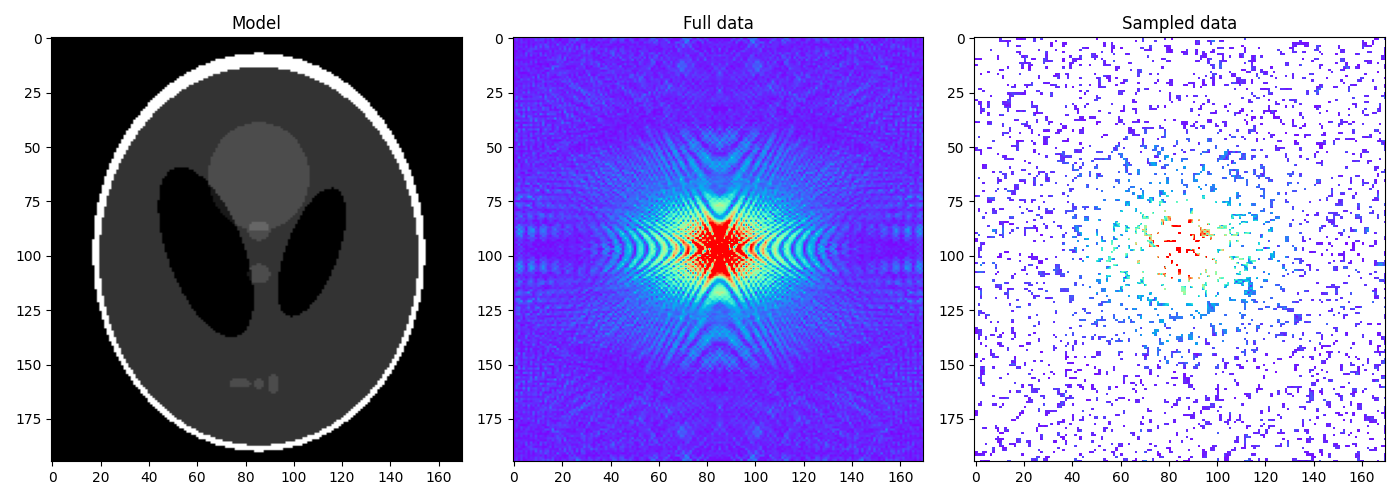
As an example, we will consider a simplified MRI experiment, where the data is created by appling a 2D Fourier Transform to the input model and by randomly sampling 60% of its values. We will use the famous BM3D as the denoiser, but any other denoiser of choice can be used instead!
Finally, whilst in the original paper, PnP is associated to the ADMM solver, subsequent
research showed that the same principle can be applied to pretty much any proximal
solver. We will show how to pass a solver of choice to our
pyproximal.optimization.pnp.PlugAndPlay solver.
import bm3d
import matplotlib.pyplot as plt
import numpy as np
import pylops
from pylops.config import set_ndarray_multiplication
from pylops.utils.metrics import snr

import pyproximal

plt.close("all")
np.random.seed(0)
set_ndarray_multiplication(False)
Let’s start by loading the famous Shepp logan phantom and creating the modelling operator
x = np.load("../testdata/shepp_logan_phantom.npy")
x = x / x.max()
ny, nx = x.shape

perc_subsampling = 0.6
nxsub = int(np.round(ny * nx * perc_subsampling))
iava = np.sort(np.random.permutation(np.arange(ny * nx))[:nxsub])
Rop = pylops.Restriction(ny * nx, iava, dtype=np.complex128)
Fop = pylops.signalprocessing.FFT2D(dims=(ny, nx))
We now create and display the data alongside the model
y = Rop * Fop * x.ravel()
yfft = Fop * x.ravel()
yfft = np.fft.fftshift(yfft.reshape(ny, nx))

ymask = Rop.mask(Fop * x.ravel())
ymask = ymask.reshape(ny, nx)
ymask.data[:] = np.fft.fftshift(ymask.data)
ymask.mask[:] = np.fft.fftshift(ymask.mask)

fig, axs = plt.subplots(1, 3, figsize=(14, 5))
axs[0].imshow(x, vmin=0, vmax=1, cmap="gray")
axs[0].set_title("Model")
axs[0].axis("tight")
axs[1].imshow(np.abs(yfft), vmin=0, vmax=1, cmap="rainbow")
axs[1].set_title("Full data")
axs[1].axis("tight")
axs[2].imshow(np.abs(ymask), vmin=0, vmax=1, cmap="rainbow")
axs[2].set_title("Sampled data")
axs[2].axis("tight")
plt.tight_layout()
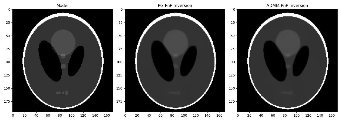
At this point we create a denoiser instance using the BM3D algorithm and use as Plug-and-Play Prior to the ADMM, PG and HQS algorithms
def callback(x, xtrue, errhist):
    errhist.append(np.linalg.norm(x - xtrue))


Op = Rop * Fop
L = np.real((Op.H * Op).eigs(neigs=1, which="LM")[0])
tau = 1.0 / L
sigma = 0.05

# BM3D denoiser
denoiser = lambda x, tau: bm3d.bm3d(
    np.real(x), sigma_psd=sigma * tau, stage_arg=bm3d.BM3DStages.HARD_THRESHOLDING
)

# ADMM-PnP
l2 = pyproximal.proximal.L2(Op=Op, b=y.ravel(), niter=50, warm=True)

errhistadmm = []
xpnpadmm = pyproximal.optimization.pnp.PlugAndPlay(
    l2,
    denoiser,
    x.shape,
    solver=pyproximal.optimization.primal.ADMM,
    tau=tau,
    x0=np.zeros(x.size, dtype=np.complex128),
    niter=40,
    show=True,
    callback=lambda xx: callback(xx, x.ravel(), errhistadmm),
)[0]
xpnpadmm = np.real(xpnpadmm.reshape(x.shape))

# PG-Pnp
l2 = pyproximal.proximal.L2(Op=Op, b=y.ravel(), niter=50, warm=True)

errhistpg = []
xpnppg = pyproximal.optimization.pnp.PlugAndPlay(
    l2,
    denoiser,
    x.shape,
    solver=pyproximal.optimization.primal.ProximalGradient,
    tau=tau,
    x0=np.zeros(x.size, dtype=np.complex128),
    niter=40,
    acceleration="fista",
    show=True,
    callback=lambda xx: callback(xx, x.ravel(), errhistpg),
)
xpnppg = np.real(xpnppg.reshape(x.shape))

# HQS-PnP
l2 = pyproximal.proximal.L2(Op=Op, b=y.ravel(), niter=50, warm=True)

tau_hqs = 1.0 / L * 0.99 ** (np.arange(40))
errhisthqs = []
xpnphqs = pyproximal.optimization.pnp.PlugAndPlay(
    l2,
    denoiser,
    x.shape,
    solver=pyproximal.optimization.primal.HQS,
    tau=tau_hqs,
    x0=np.zeros(x.size, dtype=np.complex128),
    niter=40,
    show=True,
    callback=lambda xx: callback(xx, x.ravel(), errhisthqs),
)[0]
xpnphqs = np.real(xpnphqs.reshape(x.shape))

fig, axs = plt.subplots(1, 4, sharey=True, figsize=(15, 5))
axs[0].imshow(x, vmin=0, vmax=1, cmap="gray")
axs[0].set_title("Model")
axs[0].axis("tight")
axs[1].imshow(xpnpadmm, vmin=0, vmax=1, cmap="gray")
axs[1].set_title(f"ADMM-PnP (SNR={snr(x, xpnpadmm):.2f} dB)")
axs[1].axis("tight")
axs[2].imshow(xpnppg, vmin=0, vmax=1, cmap="gray")
axs[2].set_title(f"PG-PnP (SNR={snr(x, xpnppg):.2f} dB)")
axs[2].axis("tight")
axs[3].imshow(xpnphqs, vmin=0, vmax=1, cmap="gray")
axs[3].set_title(f"HQS-PnP (SNR={snr(x, xpnphqs):.2f} dB)")
axs[3].axis("tight")
plt.tight_layout()
ADMM
-----------------------------------------------------------------
Proximal operator (f): L2
Proximal operator (g): _Denoise

tau = 1.000000e+00      niter = 40
gfirst = False          tol = None
-----------------------------------------------------------------

    Itn              x[0]                 f           g         J=f+g
     1        1.16e-02-4.31e-02j      2.216e+02   0.000e+00   2.216e+02
     2        -8.56e-03+1.85e-03j      1.145e+02   0.000e+00   1.145e+02
     3        -1.18e-02+9.03e-03j      5.280e+01   0.000e+00   5.280e+01
     4        -2.08e-02+8.42e-03j      2.375e+01   0.000e+00   2.375e+01
     5        -1.85e-02+2.41e-03j      1.123e+01   0.000e+00   1.123e+01
     6        -1.72e-02+3.36e-03j      6.032e+00   0.000e+00   6.032e+00
     7        -2.03e-02+1.95e-03j      3.873e+00   0.000e+00   3.873e+00
     8        -2.14e-02+1.05e-03j      2.922e+00   0.000e+00   2.922e+00
     9        -2.14e-02+1.05e-03j      2.446e+00   0.000e+00   2.446e+00
    10        -2.21e-02+1.19e-03j      2.195e+00   0.000e+00   2.195e+00
    11        -2.19e-02+8.32e-04j      2.044e+00   0.000e+00   2.044e+00
    21        -1.10e-02+5.21e-07j      1.528e+00   0.000e+00   1.528e+00
    31        -5.45e-03+2.59e-04j      1.440e+00   0.000e+00   1.440e+00
    32        -5.21e-03-1.91e-04j      1.440e+00   0.000e+00   1.440e+00
    33        -5.15e-03+1.40e-06j      1.436e+00   0.000e+00   1.436e+00
    34        -4.66e-03-2.16e-05j      1.438e+00   0.000e+00   1.438e+00
    35        -4.61e-03+2.61e-04j      1.437e+00   0.000e+00   1.437e+00
    36        -4.49e-03-5.95e-05j      1.437e+00   0.000e+00   1.437e+00
    37        -4.28e-03+1.17e-05j      1.437e+00   0.000e+00   1.437e+00
    38        -4.18e-03-1.52e-05j      1.428e+00   0.000e+00   1.428e+00
    39        -3.96e-03+2.16e-04j      1.426e+00   0.000e+00   1.426e+00
    40        -4.16e-03-2.48e-04j      1.424e+00   0.000e+00   1.424e+00

Iterations = 40        Total time (s) = 33.18
-----------------------------------------------------------------

ProximalGradient
---------------------------------------------------------------------------------
Proximal operator (f): L2
Proximal operator (g): _Denoise

tau = 1.00e+00          backtrack = False
beta = 0.5              epsg = 1.0              acceleration = fista
niter = 40              niterback = 100         tol = None
---------------------------------------------------------------------------------

    Itn              x[0]                  f           g       J=f+eps*g     tau
     1         5.7954e-02       6.093e+01   0.000e+00   6.093e+01  1.00e+00
     2         5.1158e-03       1.826e+01   0.000e+00   1.826e+01  1.00e+00
     3        -3.0189e-02       5.365e+00   0.000e+00   5.365e+00  1.00e+00
     4        -2.5392e-02       2.701e+00   0.000e+00   2.701e+00  1.00e+00
     5        -2.2982e-02       2.213e+00   0.000e+00   2.213e+00  1.00e+00
     6        -2.7183e-02       1.998e+00   0.000e+00   1.998e+00  1.00e+00
     7        -2.8295e-02       1.853e+00   0.000e+00   1.853e+00  1.00e+00
     8        -2.4980e-02       1.750e+00   0.000e+00   1.750e+00  1.00e+00
     9        -2.0491e-02       1.658e+00   0.000e+00   1.658e+00  1.00e+00
    10        -1.4630e-02       1.567e+00   0.000e+00   1.567e+00  1.00e+00
    11        -8.9494e-03       1.492e+00   0.000e+00   1.492e+00  1.00e+00
    21        -2.3636e-03       1.409e+00   0.000e+00   1.409e+00  1.00e+00
    31        -3.0503e-03       1.420e+00   0.000e+00   1.420e+00  1.00e+00
    32        -2.8543e-03       1.422e+00   0.000e+00   1.422e+00  1.00e+00
    33        -2.7283e-03       1.418e+00   0.000e+00   1.418e+00  1.00e+00
    34        -2.6629e-03       1.418e+00   0.000e+00   1.418e+00  1.00e+00
    35        -2.5689e-03       1.414e+00   0.000e+00   1.414e+00  1.00e+00
    36        -2.6600e-03       1.411e+00   0.000e+00   1.411e+00  1.00e+00
    37        -2.8677e-03       1.405e+00   0.000e+00   1.405e+00  1.00e+00
    38        -3.0011e-03       1.409e+00   0.000e+00   1.409e+00  1.00e+00
    39        -3.1309e-03       1.417e+00   0.000e+00   1.417e+00  1.00e+00
    40        -3.2689e-03       1.413e+00   0.000e+00   1.413e+00  1.00e+00

Iterations = 40        Total time (s) = 32.94
---------------------------------------------------------------------------------

HQS
-----------------------------------------------------------------
Proximal operator (f): L2
Proximal operator (g): _Denoise

tau = Variable  niter = 40
gfirst = True   tol = None
-----------------------------------------------------------------

    Itn              x[0]                  f           g         J=f+g
     1        1.16e-02-4.31e-02j      2.216e+02   0.000e+00   2.216e+02
     2        4.34e-03-3.12e-02j      8.100e+01   0.000e+00   8.100e+01
     3        -3.47e-03-2.25e-02j      3.553e+01   0.000e+00   3.553e+01
     4        -9.92e-03-1.76e-02j      1.844e+01   0.000e+00   1.844e+01
     5        -1.26e-02-1.50e-02j      1.089e+01   0.000e+00   1.089e+01
     6        -1.69e-02-1.34e-02j      7.097e+00   0.000e+00   7.097e+00
     7        -2.02e-02-1.24e-02j      4.968e+00   0.000e+00   4.968e+00
     8        -2.29e-02-1.12e-02j      3.687e+00   0.000e+00   3.687e+00
     9        -2.47e-02-9.67e-03j      2.877e+00   0.000e+00   2.877e+00
    10        -2.55e-02-8.86e-03j      2.353e+00   0.000e+00   2.353e+00
    11        -2.57e-02-8.19e-03j      1.996e+00   0.000e+00   1.996e+00
    21        -1.61e-02-4.78e-03j      9.498e-01   0.000e+00   9.498e-01
    31        -7.25e-03-3.01e-03j      6.810e-01   0.000e+00   6.810e-01
    32        -6.61e-03-2.93e-03j      6.653e-01   0.000e+00   6.653e-01
    33        -5.97e-03-2.88e-03j      6.514e-01   0.000e+00   6.514e-01
    34        -5.54e-03-2.77e-03j      6.378e-01   0.000e+00   6.378e-01
    35        -5.00e-03-2.82e-03j      6.258e-01   0.000e+00   6.258e-01
    36        -4.62e-03-2.82e-03j      6.156e-01   0.000e+00   6.156e-01
    37        -4.17e-03-2.63e-03j      6.048e-01   0.000e+00   6.048e-01
    38        -3.82e-03-2.56e-03j      5.947e-01   0.000e+00   5.947e-01
    39        -3.56e-03-2.50e-03j      5.853e-01   0.000e+00   5.853e-01
    40        -3.29e-03-2.51e-03j      5.753e-01   0.000e+00   5.753e-01

Iterations = 40        Total time (s) = 32.95
-----------------------------------------------------------------
Finally, the attentive reader may have noticed that in the HQS server a continuation strategy was used for the tau parameter; whilst this is strictly needed for HQS to converge, there is a consensus in the literature that also other solvers should benefit from adopting the same strategy when used with a PnP prior. This can be in fact interpreted as reducing the strength of the denoiser as iterations progress and the estimate comes closer to the true solution.
While our pyproximal.optimization.primal.ADMM solver does currently
not offer relaxation out-of-the-box, this can be achieved pretty easily
by creating an auxiliary Denoiser class with a decay parameter as
shown below.
class Denoiser:
    def __init__(self, sigma, decay):
        self.sigma = sigma
        self.decay = decay
        self.iiter = 0

    def denoise(self, x, tau):
        xden = bm3d.bm3d(
            np.real(x),
            sigma_psd=self.decay[self.iiter] * self.sigma * tau,
            stage_arg=bm3d.BM3DStages.HARD_THRESHOLDING,
        )
        self.iiter += 1
        return xden


# ADMM-PnP with relaxation
denoiser = Denoiser(sigma, decay=0.99 ** (np.arange(40)))
l2 = pyproximal.proximal.L2(Op=Op, b=y.ravel(), niter=50, warm=True)

errhistadmm1 = []
xpnpadmm1 = pyproximal.optimization.pnp.PlugAndPlay(
    l2,
    denoiser.denoise,
    x.shape,
    solver=pyproximal.optimization.primal.ADMM,
    tau=tau,
    x0=np.zeros(x.size, dtype=np.complex128),
    niter=40,
    show=True,
    callback=lambda xx: callback(xx, x.ravel(), errhistadmm1),
)[0]
xpnpadmm1 = np.real(xpnpadmm1.reshape(x.shape))

fig, axs = plt.subplots(1, 3, sharey=True, figsize=(15, 5))
axs[0].imshow(x, vmin=0, vmax=1, cmap="gray")
axs[0].set_title("Model")
axs[0].axis("tight")
axs[1].imshow(xpnpadmm, vmin=0, vmax=1, cmap="gray")
axs[1].set_title(f"ADMM-PnP (SNR={snr(x, xpnpadmm):.2f} dB)")
axs[1].axis("tight")
axs[2].imshow(xpnpadmm1, vmin=0, vmax=1, cmap="gray")
axs[2].set_title(f"ADMM-PnP with rel. (SNR={snr(x, xpnpadmm1):.2f} dB)")
axs[2].axis("tight")
plt.tight_layout()
ADMM
-----------------------------------------------------------------
Proximal operator (f): L2
Proximal operator (g): _Denoise

tau = 1.000000e+00      niter = 40
gfirst = False          tol = None
-----------------------------------------------------------------

    Itn              x[0]                 f           g         J=f+g
     1        1.16e-02-4.31e-02j      2.216e+02   0.000e+00   2.216e+02
     2        -8.56e-03+1.85e-03j      1.145e+02   0.000e+00   1.145e+02
     3        -9.34e-03+9.10e-03j      5.266e+01   0.000e+00   5.266e+01
     4        -2.23e-02+8.06e-03j      2.353e+01   0.000e+00   2.353e+01
     5        -2.25e-02+3.45e-03j      1.096e+01   0.000e+00   1.096e+01
     6        -1.70e-02+3.01e-03j      5.774e+00   0.000e+00   5.774e+00
     7        -1.96e-02+1.42e-03j      3.616e+00   0.000e+00   3.616e+00
     8        -2.07e-02+1.28e-03j      2.642e+00   0.000e+00   2.642e+00
     9        -2.17e-02+1.32e-03j      2.142e+00   0.000e+00   2.142e+00
    10        -2.14e-02+8.46e-04j      1.851e+00   0.000e+00   1.851e+00
    11        -2.19e-02+2.17e-03j      1.673e+00   0.000e+00   1.673e+00
    21        -1.18e-02+2.35e-04j      9.945e-01   0.000e+00   9.945e-01
    31        -5.19e-03+2.15e-04j      7.108e-01   0.000e+00   7.108e-01
    32        -4.98e-03+1.95e-04j      6.927e-01   0.000e+00   6.927e-01
    33        -4.50e-03+1.72e-04j      6.773e-01   0.000e+00   6.773e-01
    34        -4.11e-03-1.19e-05j      6.620e-01   0.000e+00   6.620e-01
    35        -4.29e-03+2.96e-04j      6.469e-01   0.000e+00   6.469e-01
    36        -4.09e-03+2.30e-04j      6.334e-01   0.000e+00   6.334e-01
    37        -3.53e-03-5.17e-05j      6.211e-01   0.000e+00   6.211e-01
    38        -3.26e-03+4.10e-05j      6.101e-01   0.000e+00   6.101e-01
    39        -3.31e-03+6.49e-05j      6.010e-01   0.000e+00   6.010e-01
    40        -3.06e-03+2.28e-04j      5.908e-01   0.000e+00   5.908e-01

Iterations = 40        Total time (s) = 33.02
-----------------------------------------------------------------
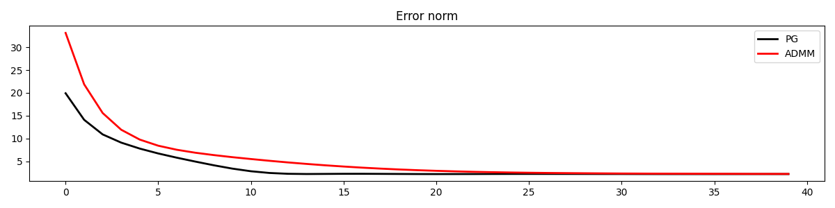
Let’s finally compare the error convergence of the four variations of PnP
plt.figure(figsize=(12, 3))
plt.semilogy(errhistadmm, "k", lw=2, label="ADMM")
plt.semilogy(errhistpg, "r", lw=2, label="PG")
plt.semilogy(errhisthqs, "b", lw=2, label="HQS")
plt.semilogy(errhistadmm1, "--b", lw=2, label="ADMM with rel.")
plt.title("Error norm")
plt.legend()
plt.tight_layout()
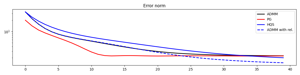
This final results clearly shows the importance of relaxation also for ADMM.
Total running time of the script: (2 minutes 13.543 seconds)