Non-rigid structure-from-motion (NRSfM)

In computer vision, structure-from-motion (SfM) is an imaging technique for estimating three-dimensional structures from two-dimensional images. Theoretically, the problem is generally well-posed when considering rigid objects, meaning that the objects do not move or deform in the scene. However, non-static scenes are still relevant and have gained increased popularity among researchers in recent years. This is known as non-rigid structure-from-motion.

In this tutorial, we will consider motion capture (MOCAP). This is a special case, where we use images from multiple camera views to compute the 3D positions of specifically designed markers that track the motion of a person (or object) performing various tasks.

Non-rigid shapes

To make the problem well-posed, one has to control the complexity of the deformations using some minor assumptions on the possible space of object shapes. This is not a weird thing to do: consider e.g. the human body, we have different joints that bend and turn in a finite amount of ways; the skeleton itself is rigid and not capable of such deformations. For this reason, Bregler et al. 1 suggested that all movements (or shapes) can be represented by a low-dimensional basis. In the context of motion capture, this means that every movement a person does can be considered a combination of core movements (or basis shapes).

Mathematically speaking, this translates to any motion being a linear combination of the basis shapes, i.e. assuming there are \(K\) basis shapes, any non-rigid shape \(X_i\) can be written as

\[X_i = \sum_{i=1}^K c_{ik}B_k\]

where \(c_{ik}\) are the basis coefficients and \(B_k\) are the basis shapes. Here, \(X_i\) is a \(3\times N\) matrix where each column is a point in 3D space.

The CMU MOCAP dataset

Let us first try to understand the data we are given. We will use the Pickup instance from the CMU MOCAP dataset, which depicts a person picking something up from the floor.

import matplotlib.pyplot as plt
import matplotlib.animation as animation
import numpy as np
import scipy as sp


plt.close('all')
np.random.seed(0)
data = np.load('../testdata/mocap.npz', allow_pickle=True)
X_gt = data['X_gt']
markers = data['markers'].item()

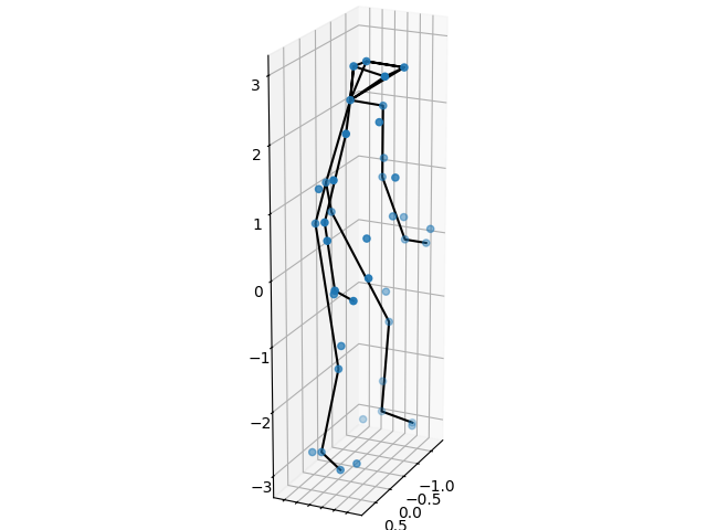
First we view the first 3D poses. In order to easily visualize the person, we draw a skeleton between the markers corresponding to certain body parts. Note that these are not used in any other way.

def plot_first_3d_pose(ax, X, color='b', marker='o', linecolor='k'):
    ax.scatter(X[0, :], X[1, :], X[2, :], color, marker=marker)
    for j, ind in enumerate(markers.values()):
        ax.plot(X[0, ind], X[1, ind], X[2, ind], '-', color=linecolor)
    ax.set_box_aspect(np.ptp(X[:3, :], axis=1))
    ax.view_init(20, 25)


fig = plt.figure()
ax = fig.add_subplot(projection='3d')
plot_first_3d_pose(ax, X_gt)
plt.tight_layout()

Now, we turn the attention to the data the algorithm is given, which is a sequence of 2D images from varying views. The goal is to recreate the 3D points, such as in the example above, from all timestamps.

M = data['M']
F = int(X_gt.shape[0] / 3)


def _update(f: int):
    X = M[2 * f:2 * f + 2, :]
    lines[0].set_data(X[0, :], X[1, :])
    for j, ind in enumerate(markers.values()):
        lines[j + 1].set_data(X[0, ind], X[1, ind])
    return lines


fig, ax = plt.subplots()
lines = ax.plot([], [], 'r.')
for _ in range(len(markers)):
    lines.append(ax.plot([], [], 'k-')[0])
ax.set(xlim=(-2.5, 2.5), ylim=(-3.5, 3.5))
ax.set_aspect('equal')

ani = animation.FuncAnimation(fig, _update, F, interval=25, blit=True)

Once Loop Reflect

Note that these are the 2D image correspondences and that the image view is constantly changing as it is spinning around. Such motion can be modeled with orthographic cameras, which we will discuss next.

Orthographic projections

Assuming that we know the pose of the camera from which the image was taken the corresponding 2D image point can be obtained. In the case of rotations, we assume the cameras are orthographic, meaning that the image points \(x_i\) are obtained from the relation

\[x_i = R_iX_i\]

where \(R_i\) is a \(2\times 3\) matrix fulfilling \(R_iR_i^T=I\). Essentially, the \(R_i\) matrices consists of the top two rows of the corresponding rotation matrix.

Now, the task at hand is essentially the inverse problem: to reconstruct the 3D points for each point in time from these 2D images.

Treating NRSfM as a low-rank factorization problem

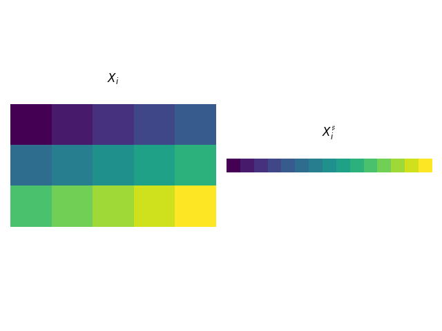
One of the main novelties of the paper by Dai et al. 2 is to reshape and stack the non-rigid shapes \(X_i\) in a way that allows us to treat the problem using methods from low-rank factorization. This is done in the following way: first concatenate all rows of \(X_i\) creating a vector \(X^\sharp_i\) of size \(1\times 3N\). Secondly, assuming there are in total \(F\) non-rigid shapes we create the matrix \(X^\sharp\) of size \(F\times 3N\) by stacking all \(X^\sharp_i\). This enables us to decompose the newly created matrix \(X^\sharp=CB^\sharp\) in the low-rank factors consisting of the shape coefficients \(C\) and the basis shapes \(B^\sharp\) (constructed in the same way as \(X^\sharp\)).

Now, let us implement and visualize this approach.

def stack(X: np.ndarray):
    return np.hstack((X[::3, :], X[1::3, :], X[2::3, :]))


Xi = np.arange(15).reshape((3, 5))
fig, ax = plt.subplots(1, 2)
ax[0].matshow(Xi)
ax[0].set_title(r'$X_i$')
ax[0].axis('off')
ax[1].matshow(stack(Xi))
ax[1].set_title(r'$X_i^\sharp$')
ax[1].axis('off')
plt.tight_layout()

Furthermore, we introduce the inverse operation, such that \(X=\mathcal{U}(X^\sharp)\), where \(\mathcal{U}\) is the “unstacking” operator.

def unstack(Xs: np.ndarray):
    """Inverse operation of stack."""
    m, n = Xs.shape
    m *= 3
    n //= 3
    X = np.zeros((m, n), dtype=Xs.dtype)
    X[::3] = Xs[:, :n]
    X[1::3] = Xs[:, n:2*n]
    X[2::3] = Xs[:, 2*n:3*n]
    return X

In many cases, the necessary amount of basis shapes is not known a priori. Therefore, a suitable objective to try to minimize is

\[\argmin_X \mu \rank(X^\sharp) + \frac{1}{2}\sum_{i=1}^F\|R_iX_i - x_i\|_2^2\]

or, equivalently,

\[\argmin_X \mu \rank(X^\sharp) + \frac{1}{2}\|RX - M\|_F^2\]

where \(R\) is a block-diagonal matrix with \(R_i\) on the main diagonal, whereas \(X\) and \(M\) are the concatenations of \(X_i\) and \(x_i\), respectively.

Since the rank function is non-convex and discontinuous, it is often replaced by a relaxation. In 2 the nuclear norm \(\|\cdot\|_{*}\) was used, i.e. we seek to minimize

\[\argmin_X \mu \|X^\sharp\|_{*} + \frac{1}{2}\|RX - M\|_F^2 \; .\]

There are some theoretical justifications for this specific choice of relaxation, e.g. the nuclear norm is the convex envelope of the rank function under curtain assumptions 3.

Solving the relaxed problem

We will now show how to solve this problem using splitting schemes. Specifically, we will use pyproximal.ADMM and re-write the objective as

\[\argmin_{X, Z} \mu \|Z^\sharp\|_{*} + \frac{1}{2}\|RX - M\|_F^2,\]

and add the constraint \(X=Z\). This way, the proximal operators are simply those of the (stacked) nuclear norm and the Frobenius norm. We implement these next:

from pyproximal.ProxOperator import _check_tau
from pyproximal import Nuclear, ProxOperator


class BlockDiagFrobenius(ProxOperator):
    r"""Proximal operator for 1/2 * ||RX - M||_F^2 where R is block-diagonal.
    Note: You could also wrap pyproximal.L2, but this class is used here in
    this tutorial to increase legibility.
    """
    def __init__(self, dim, R, M):
        super().__init__(None, False)
        self.dim = dim
        self.R = R
        self.M = M

    def __call__(self, x):
        X = x.reshape(self.dim)
        return 0.5 * np.linalg.norm(self.R @ X - self.M, 'fro') ** 2

    @_check_tau
    def prox(self, x, tau):
        X = x.reshape(self.dim)
        Y = np.zeros_like(X)
        for f, Rf in enumerate(self.R):
            Y[3 * f: 3 * f + 3, :] = np.linalg.solve(
                tau * Rf.T @ Rf + np.eye(3),
                tau * Rf.T @ self.M[2 * f:2 * f + 2, :] + X[3 * f: 3 * f + 3, :]
            )
        return Y.flatten()


class StackedNuclear(Nuclear):
    r"""Proximal operator for the stacked nuclear norm."""
    def __init__(self, dim, sigma=1.):
        super().__init__(dim, sigma)
        self.unstacked_dim = (dim[0] * 3, dim[1] // 3)

    def __call__(self, x):
        X = stack(x.reshape(self.unstacked_dim))
        return super().__call__(X.ravel())

    def prox(self, x, tau):
        X = stack(x.reshape(self.unstacked_dim))
        x = super().prox(X.ravel(), tau)
        X = unstack(x.reshape(self.dim))
        return X.ravel()

Now we are ready to solve the problem using ADMM.

from pyproximal.optimization.primal import ADMM


mu = 1
R = data['R']
Rblk = sp.linalg.block_diag(*R)
M = Rblk @ X_gt
N = M.shape[1]
normal_size = (3*F, N)
stacked_size = (F, 3*N)
X0 = np.zeros(normal_size)
proxf = BlockDiagFrobenius(normal_size, R, M)
proxg = StackedNuclear(stacked_size, mu)
X_rec = ADMM(proxf, proxg, x0=X0.flatten(), tau=0.9, niter=200)[0]
X_rec = X_rec.reshape(normal_size)

Let us compare the results with the ground truth data.

fig = plt.figure()
ax = fig.add_subplot(projection='3d')
plot_first_3d_pose(ax, X_gt)
plot_first_3d_pose(ax, X_rec, color='r', marker='v', linecolor='r')
plt.tight_layout()

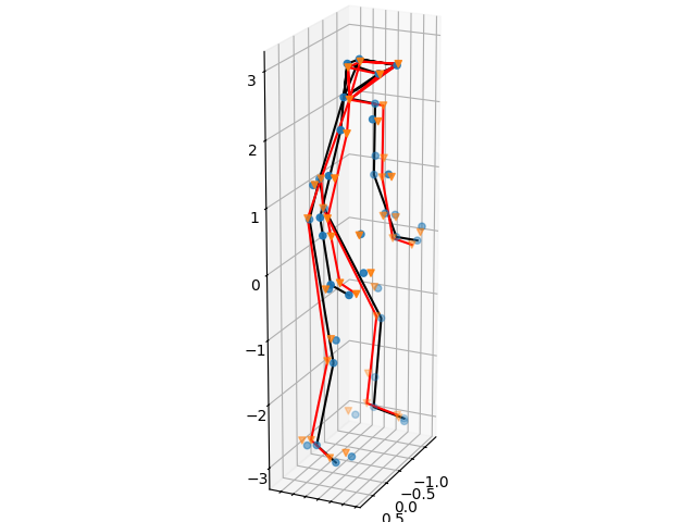
Furthermore, we compute some statistics on the reconstruction performance. You can vary the regulation strength \(\mu\) to see if you can achieve better performance yourself!

print(f'Datafit: {np.linalg.norm(Rblk @ X_rec - M, "fro")}')
print(f'Distance to GT: {np.linalg.norm(X_rec - X_gt, "fro")}')

Datafit: 4.075726006631892
Distance to GT: 12.609437571288561

One issue with the nuclear norm is that you have the hyperparameter \(\mu\) that regulates the impact of the datafit vs. model assumption. When \(\mu=0\) the datafit is perfect, but there would be no enforcement of the basis shapes, leading to severe over-fitting. On the other end, as \(\mu\to\infty\) the reconstruction turns towards the zero matrix, thus completely ignoring the given data.

Later publications have tried to mitigate this issue, and have shown that the weighted nuclear norm performs even better when the weights are selected with care 4. Other non-convex relaxations show similar results 5.

References

1

C. Bregler, A. Hertzmann, and H. Biermann. Recovering non-rigid 3d shape from image streams. In The IEEE Conference on Computer Vision and Pattern Recognition (CVPR), 2000.

2(1,2)

Y. Dai, H. Li, and M. He. A simple prior-free method for non-rigid structure-from-motion factorization. International Journal of Computer Vision, 107(2):101–122, 2014.

3

M. Fazel, H. Hindi, and S. P. Boyd. A rank minimization heuristic with application to minimum order system approximation. In the Proceedings of the American Control Conference (ACC), 2001.

4

S. Kumar. Non-rigid structure from motion: Prior-free factorization method revisited. In The IEEE Winter Conference on Applications of Computer Vision (WACV), 2020.

5

M. Valtonen Örnhag and C. Olsson. A unified optimization framework for low-rank inducing penalties. In the Proceedings of the IEEE/CVF conference on computer vision and pattern recognition (CVPR), 2020.