 PyProximal
Note
Go to the end to download the full example code.
Low-Rank completion via SVD
In this tutorial we will present an example of low-rank matrix completion. Contrarily to most of the examples in this library (and PyLops), the regularizer is here applied to a matrix, which is obtained by reshaping the model vector that we wish to solve for.
In this example we will consider the following forward problem:
where \(\mathbf{R}\) is a restriction operator, which applied to \(\mathbf{x}=\operatorname{vec}(\mathbf{X})\), the vectorized version of a 2d image of size \(n \times m\), selects a reasonably small number of samples \(p \ll nm\) that form the vector \(\mathbf{y}\). Note that any other modelling operator could be used here, for example a 2D convolutional operator in the case of deblurring or a 2D FFT plus restriction in the case of MRI scanning.
The problem we want to solve can be mathematically described as:
or
where \(\|\mathbf{X}\|_*=\sum_i \sigma_i\) is the nuclear norm of \(\mathbf{X}\) (i.e., the sum of the singular values).
import matplotlib.pyplot as plt

# sphinx_gallery_thumbnail_number = 2
import numpy as np
import pylops
from scipy import datasets

import pyproximal

plt.close("all")
np.random.seed(0)
Let’s start by loading a sample image
We can now define a pylops.Restriction operator and look at how
the singular values of our image change when we remove some of its sample.
# Restriction operator
sub = 0.4
nsub = int(ny * nx * sub)
iava = np.random.permutation(np.arange(ny * nx))[:nsub]

Rop = pylops.Restriction(ny * nx, iava)

# Data
y = Rop * X.ravel()

# Masked data
Y = (Rop.H * Rop * X.ravel()).reshape(ny, nx)

# SVD of true and masked data
Ux, Sx, Vhx = np.linalg.svd(X, full_matrices=False)
Uy, Sy, Vhy = np.linalg.svd(Y, full_matrices=False)

plt.figure()
plt.semilogy(Sx, "k", label=r"$||X||_*$=%.2f" % np.sum(Sx))
plt.semilogy(Sy, "r", label=r"$||Y||_*$=%.2f" % np.sum(Sy))
plt.legend()
plt.tight_layout()
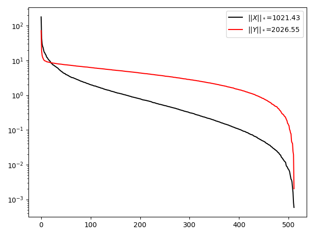
We observe that removing some samples from the image has led to an overall increase in the singular values of \(\mathbf{X}\), especially those that are originally very small. As a consequence the nuclear norm of \(\mathbf{Y}\) (the masked image) is larger than that of \(\mathbf{X}\).
Let’s now set up the inverse problem using the Proximal gradient algorithm
mu = 0.8
f = pyproximal.L2(Rop, y)
g = pyproximal.Nuclear((ny, nx), mu)

Xpg = pyproximal.optimization.primal.ProximalGradient(
    f, g, np.zeros(ny * nx), acceleration="vandenberghe", tau=1.0, niter=100, show=True
)
Xpg = Xpg.reshape(ny, nx)

# Recompute SVD and see how the singular values look like
Upg, Spg, Vhpg = np.linalg.svd(Xpg, full_matrices=False)
ProximalGradient
---------------------------------------------------------------------------------
Proximal operator (f): L2
Proximal operator (g): Nuclear

tau = 1.00e+00          backtrack = False
beta = 0.5              epsg = 1.0              acceleration = vandenberghe
niter = 100             niterback = 100         tol = None
---------------------------------------------------------------------------------

    Itn           x[0]              f           g       J=f+eps*g     tau
     1         2.8023e-01       9.762e+01   1.314e+03   1.412e+03  1.00e+00
     2         2.7987e-01       9.629e+01   1.223e+03   1.319e+03  1.00e+00
     3         2.8967e-01       9.359e+01   1.129e+03   1.222e+03  1.00e+00
     4         2.9403e-01       9.019e+01   1.035e+03   1.125e+03  1.00e+00
     5         3.0007e-01       8.645e+01   9.438e+02   1.030e+03  1.00e+00
     6         3.0735e-01       8.300e+01   8.565e+02   9.395e+02  1.00e+00
     7         3.1687e-01       8.025e+01   7.742e+02   8.545e+02  1.00e+00
     8         3.1686e-01       7.828e+01   6.988e+02   7.770e+02  1.00e+00
     9         3.1327e-01       7.674e+01   6.331e+02   7.098e+02  1.00e+00
    10         3.1341e-01       7.566e+01   5.796e+02   6.553e+02  1.00e+00
    11         3.1495e-01       7.515e+01   5.400e+02   6.151e+02  1.00e+00
    21         3.0637e-01       7.479e+01   4.884e+02   5.631e+02  1.00e+00
    31         3.1219e-01       7.520e+01   4.869e+02   5.621e+02  1.00e+00
    41         3.1101e-01       7.515e+01   4.868e+02   5.620e+02  1.00e+00
    51         3.1119e-01       7.518e+01   4.868e+02   5.620e+02  1.00e+00
    61         3.1124e-01       7.518e+01   4.868e+02   5.620e+02  1.00e+00
    71         3.1114e-01       7.518e+01   4.868e+02   5.620e+02  1.00e+00
    81         3.1122e-01       7.518e+01   4.868e+02   5.620e+02  1.00e+00
    91         3.1117e-01       7.518e+01   4.868e+02   5.620e+02  1.00e+00
    92         3.1117e-01       7.518e+01   4.868e+02   5.620e+02  1.00e+00
    93         3.1118e-01       7.518e+01   4.868e+02   5.620e+02  1.00e+00
    94         3.1118e-01       7.518e+01   4.868e+02   5.620e+02  1.00e+00
    95         3.1119e-01       7.518e+01   4.868e+02   5.620e+02  1.00e+00
    96         3.1119e-01       7.518e+01   4.868e+02   5.620e+02  1.00e+00
    97         3.1119e-01       7.518e+01   4.868e+02   5.620e+02  1.00e+00
    98         3.1120e-01       7.518e+01   4.868e+02   5.620e+02  1.00e+00
    99         3.1120e-01       7.518e+01   4.868e+02   5.620e+02  1.00e+00
   100         3.1120e-01       7.518e+01   4.868e+02   5.620e+02  1.00e+00

Iterations = 100        Total time (s) = 9.97
---------------------------------------------------------------------------------
Let’s do the same with the constrained version
mu1 = 0.8 * np.sum(Sx)
g = pyproximal.proximal.NuclearBall((ny, nx), mu1)

Xpgc = pyproximal.optimization.primal.ProximalGradient(
    f, g, np.zeros(ny * nx), acceleration="vandenberghe", tau=1.0, niter=100, show=True
)
Xpgc = Xpgc.reshape(ny, nx)

# Recompute SVD and see how the singular values look like
Upgc, Spgc, Vhpgc = np.linalg.svd(Xpgc, full_matrices=False)
ProximalGradient
---------------------------------------------------------------------------------
Proximal operator (f): L2
Proximal operator (g): NuclearBall

tau = 1.00e+00          backtrack = False
beta = 0.5              epsg = 1.0              acceleration = vandenberghe
niter = 100             niterback = 100         tol = None
---------------------------------------------------------------------------------

    Itn           x[0]              f           g       J=f+eps*g     tau
     1         1.9070e-01       1.162e+03   0.000e+00   1.162e+03  1.00e+00
     2         2.5326e-01       6.432e+02   0.000e+00   6.432e+02  1.00e+00
     3         2.8651e-01       3.437e+02   1.000e+00   3.447e+02  1.00e+00
     4         3.0491e-01       1.802e+02   0.000e+00   1.802e+02  1.00e+00
     5         3.1273e-01       9.470e+01   1.000e+00   9.570e+01  1.00e+00
     6         3.1584e-01       5.078e+01   1.000e+00   5.178e+01  1.00e+00
     7         3.1794e-01       2.813e+01   0.000e+00   2.813e+01  1.00e+00
     8         3.1890e-01       1.623e+01   1.000e+00   1.723e+01  1.00e+00
     9         3.1883e-01       9.769e+00   0.000e+00   9.769e+00  1.00e+00
    10         3.1903e-01       6.129e+00   0.000e+00   6.129e+00  1.00e+00
    11         3.1998e-01       3.995e+00   1.000e+00   4.995e+00  1.00e+00
    21         3.2519e-01       1.995e-01   0.000e+00   1.995e-01  1.00e+00
    31         3.2543e-01       2.777e-02   1.000e+00   1.028e+00  1.00e+00
    41         3.2545e-01       4.893e-03   1.000e+00   1.005e+00  1.00e+00
    51         3.2547e-01       7.274e-04   0.000e+00   7.274e-04  1.00e+00
    61         3.2548e-01       4.032e-05   0.000e+00   4.032e-05  1.00e+00
    71         3.2549e-01       7.626e-09   1.000e+00   1.000e+00  1.00e+00
    81         3.2549e-01       9.189e-09   0.000e+00   9.189e-09  1.00e+00
    91         3.2549e-01       1.053e-08   0.000e+00   1.053e-08  1.00e+00
    92         3.2549e-01       9.221e-08   1.000e+00   1.000e+00  1.00e+00
    93         3.2549e-01       1.089e-08   0.000e+00   1.089e-08  1.00e+00
    94         3.2549e-01       1.074e-08   0.000e+00   1.074e-08  1.00e+00
    95         3.2549e-01       1.064e-08   0.000e+00   1.064e-08  1.00e+00
    96         3.2549e-01       1.061e-08   0.000e+00   1.061e-08  1.00e+00
    97         3.2549e-01       1.061e-08   0.000e+00   1.061e-08  1.00e+00
    98         3.2549e-01       1.062e-08   0.000e+00   1.062e-08  1.00e+00
    99         3.2549e-01       1.064e-08   0.000e+00   1.064e-08  1.00e+00
   100         3.2549e-01       1.066e-08   0.000e+00   1.066e-08  1.00e+00

Iterations = 100        Total time (s) = 11.08
---------------------------------------------------------------------------------
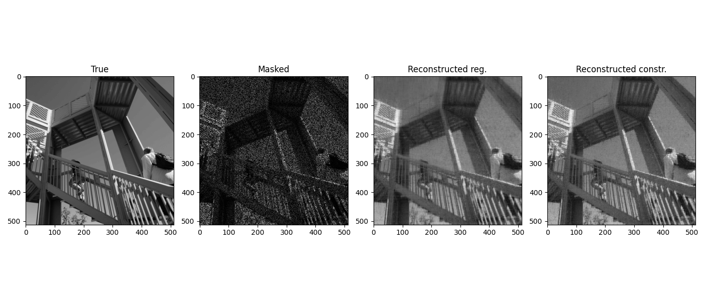
We now display the reconstructed images
fig, axs = plt.subplots(1, 4, figsize=(14, 6))
axs[0].imshow(X, cmap="gray")
axs[0].set_title("True")
axs[1].imshow(Y, cmap="gray")
axs[1].set_title("Masked")
axs[2].imshow(Xpg, cmap="gray")
axs[2].set_title("Reconstructed reg.")
axs[3].imshow(Xpgc, cmap="gray")
axs[3].set_title("Reconstructed constr.")
fig.tight_layout()
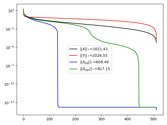
And finally we compare the singular values of the original image, the masked image and the reconstructed images
plt.figure()
plt.semilogy(Sx, "k", label=r"$||X||_*$=%.2f" % np.sum(Sx))
plt.semilogy(Sy, "r", label=r"$||Y||_*$=%.2f" % np.sum(Sy))
plt.semilogy(Spg, "b", label=r"$||X_{pg}||_*$=%.2f" % np.sum(Spg))
plt.semilogy(Spgc, "g", label=r"$||X_{pgc}||_*$=%.2f" % np.sum(Spgc))
plt.legend()
plt.tight_layout()
Total running time of the script: (0 minutes 22.272 seconds)