Note
Go to the end to download the full example code.
IHT, ISTA, FISTA, AA-ISTA, and TWIST for Compressive sensing
In this example we want to compare five popular solvers in compressive
sensing problem, namely IHT, ISTA, FISTA, AA-ISTA, and TwIST. The first three can
be implemented using the same solver, namely the
pyproximal.optimization.primal.ProximalGradient, whilst the latter
two are implemented using the pyproximal.optimization.primal.AndersonProximalGradient and
pyproximal.optimization.primal.TwIST solvers, respectively
The IHT solver tries to solve the following unconstrained problem with a L0Ball regularization term:
The other solvers try instead to solve an unconstrained problem with a L1 regularization term:
however their convergence speed is different, which is something we want to focus in this tutorial.
Let’s start by creating a dense mixing matrix and a sparse signal. Note that the mixing matrix leads to an underdetermined system of equations (\(N < M\)) so being able to add some extra prior information regarding the sparsity of our desired model is essential to be able to invert such a system.
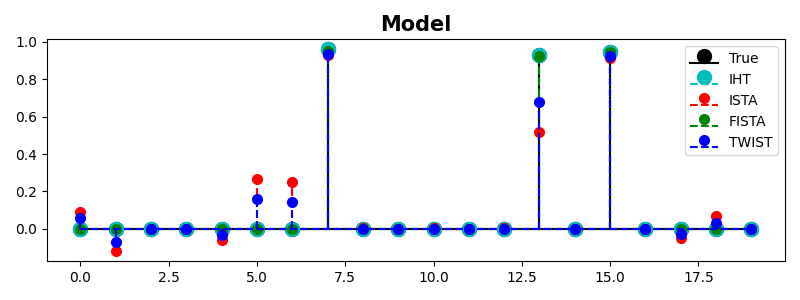
We try now to recover the sparse signal with our 4 different solvers
L = np.abs((Aop.H * Aop).eigs(1)[0])
tau = 0.95 / L
eps = 5e-3
maxit = 300

# IHT
l0 = pyproximal.proximal.L0Ball(3)
l2 = pyproximal.proximal.L2(Op=Aop, b=y)
costf1 = []
x_iht = pyproximal.optimization.primal.ProximalGradient(
    l2,
    l0,
    tau=tau,
    x0=np.zeros(M),
    epsg=eps,
    niter=maxit,
    acceleration="fista",
    show=False,
)

# ISTA
l1 = pyproximal.proximal.L1()
l2 = pyproximal.proximal.L2(Op=Aop, b=y)
costi = []
x_ista = pyproximal.optimization.primal.ProximalGradient(
    l2,
    l1,
    tau=tau,
    x0=np.zeros(M),
    epsg=eps,
    niter=maxit,
    show=False,
    callback=lambda x: callback(x, l2, l1, eps, costi),
)
niteri = len(costi)

# FISTA
l1 = pyproximal.proximal.L1()
l2 = pyproximal.proximal.L2(Op=Aop, b=y)
costf = []
x_fista = pyproximal.optimization.primal.ProximalGradient(
    l2,
    l1,
    tau=tau,
    x0=np.zeros(M),
    epsg=eps,
    niter=maxit,
    acceleration="fista",
    show=False,
    callback=lambda x: callback(x, l2, l1, eps, costf),
)
niterf = len(costf)

# Anderson accelerated ISTA
l1 = pyproximal.proximal.L1()
l2 = pyproximal.proximal.L2(Op=Aop, b=y)
costa = []
x_ander = pyproximal.optimization.primal.AndersonProximalGradient(
    l2,
    l1,
    tau=tau,
    x0=np.zeros(M),
    epsg=eps,
    niter=maxit,
    nhistory=5,
    show=False,
    callback=lambda x: callback(x, l2, l1, eps, costa),
)
nitera = len(costa)


# TWIST (Note that since the smallest eigenvalue is zero, we arbitrarily
# choose a small value for the solver to converge stably)
l1 = pyproximal.proximal.L1(sigma=eps)
eigs = (Aop.H * Aop).eigs()
eigs = (np.abs(eigs[0]), 5e-1)
x_twist, costt = pyproximal.optimization.primal.TwIST(
    l1, Aop, y, eigs=eigs, x0=np.zeros(M), niter=maxit, show=False, returncost=True
)

fig, ax = plt.subplots(1, 1, figsize=(8, 3))
m, s, b = ax.stem(x, linefmt="k", basefmt="k", markerfmt="ko", label="True")
plt.setp(m, markersize=10)
m, s, b = ax.stem(x_iht, linefmt="--c", basefmt="--c", markerfmt="co", label="IHT")
plt.setp(m, markersize=10)
m, s, b = ax.stem(x_ista, linefmt="--r", basefmt="--r", markerfmt="ro", label="ISTA")
plt.setp(m, markersize=7)
m, s, b = ax.stem(x_fista, linefmt="--g", basefmt="--g", markerfmt="go", label="FISTA")
plt.setp(m, markersize=7)
m, s, b = ax.stem(
    x_ander, linefmt="--m", basefmt="--m", markerfmt="mo", label="AA-ISTA"
)
plt.setp(m, markersize=7)
m, s, b = ax.stem(x_twist, linefmt="--b", basefmt="--b", markerfmt="bo", label="TWIST")
plt.setp(m, markersize=7)
ax.set_title("Model", size=15, fontweight="bold")
ax.legend()
plt.tight_layout()
Finally, let’s compare the converge behaviour of the different algorithms
fig, ax = plt.subplots(1, 1, figsize=(8, 4))
ax.loglog(costi, "r", lw=2, label=r"$x_{ISTA} (niter=%d)$" % niteri)
ax.loglog(costf, "g", lw=2, label=r"$x_{FISTA} (niter=%d)$" % niterf)
ax.loglog(costa, "m", lw=2, label=r"$x_{AA-ISTA} (niter=%d)$" % nitera)
ax.loglog(costt, "b", lw=2, label=r"$x_{TWIST} (niter=%d)$" % maxit)
ax.set_title("Cost function", size=15, fontweight="bold")
ax.set_xlabel("Iteration")
ax.legend()
ax.grid(True, which="both")
plt.tight_layout()
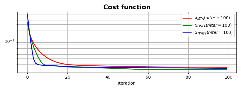
To conclude, given the nature of the problem (small number of non-zero coefficients), the IHT solver shows the fastest convergence - note that we do not display the cost function since this is a constrained problem. This is however greatly influenced by the fact that we assume exact knowledge of the number of non-zero coefficients. When this information is not available, IHT may become suboptimal. In this case the FISTA or AA-ISTA solvers should always be preferred (over ISTA) and TwIST represents an alternative worth checking.
Total running time of the script: (0 minutes 0.652 seconds)