Adaptive Primal-Dual¶

This tutorial compares the traditional Chambolle-Pock Primal-dual algorithm with the Adaptive Primal-Dual Hybrid Gradient of Goldstein and co-authors.

By adaptively changing the step size in the primal and the dual directions, this algorithm shows faster convergence, which is of great importance for some of the problems that the Primal-Dual algorithm can solve - especially those with an expensive proximal operator.

For this example, we consider a simple denoising problem.

import matplotlib.pyplot as plt
import numpy as np
import pylops
from skimage.data import camera

import pyproximal

plt.close("all")
np.random.seed(10)


def callback(x, f, g, K, cost, xtrue, err):
    cost.append(f(x) + g(K.matvec(x)))
    err.append(np.linalg.norm(x - xtrue))

Let’s start by loading a sample image and adding some noise

# Load image
img = camera()
ny, nx = img.shape

# Add noise
sigman = 20
n = np.random.normal(0, sigman, img.shape)
noise_img = img + n

We can now define a pylops.Gradient operator as well as the different proximal operators to be passed to our solvers

# Gradient operator
sampling = 1.0
Gop = pylops.Gradient(
    dims=(ny, nx), sampling=sampling, edge=False, kind="forward", dtype="float64"
)
L = 8.0 / sampling**2  # maxeig(Gop^H Gop)

# L2 data term
lamda = 0.04
l2 = pyproximal.L2(b=noise_img.ravel(), sigma=lamda)

# L1 regularization (isotropic TV)
l1iso = pyproximal.L21(ndim=2)

To start, we solve our denoising problem with the original Primal-Dual algorithm

# Primal-dual
tau = 0.95 / np.sqrt(L)
mu = 0.95 / np.sqrt(L)

cost_fixed = []
err_fixed = []
iml12_fixed = pyproximal.optimization.primaldual.PrimalDual(
    l2,
    l1iso,
    Gop,
    tau=tau,
    mu=mu,
    theta=1.0,
    x0=np.zeros_like(img.ravel()),
    gfirst=False,
    niter=300,
    show=True,
    callback=lambda x: callback(x, l2, l1iso, Gop, cost_fixed, img.ravel(), err_fixed),
)
iml12_fixed = iml12_fixed.reshape(img.shape)

PrimalDual
-------------------------------------------------------------------------------------
Proximal operator (f): L2
Proximal operator (g): L21
Linear operator (A): Gradient
Additional vector (z): None

tau = 0.335876  mu = 0.335876   theta = 1.00e+00
tol = None      niter = 300
-------------------------------------------------------------------------------------

    Itn           x[0]                 f            g          z^x       J=f+g+z^x
       3.0044e+00          1.1465e+08  1.3295e+05   0.0000e+00   1.1478e+08
       5.8125e+00          1.1169e+08  1.3834e+05   0.0000e+00   1.1183e+08
       8.4231e+00          1.0883e+08  1.2165e+05   0.0000e+00   1.0895e+08
       1.0891e+01          1.0605e+08  1.1152e+05   0.0000e+00   1.0616e+08
       1.3292e+01          1.0333e+08  1.1084e+05   0.0000e+00   1.0344e+08
       1.5663e+01          1.0069e+08  1.1422e+05   0.0000e+00   1.0080e+08
       1.8038e+01          9.8109e+07  1.1861e+05   0.0000e+00   9.8227e+07
       2.0425e+01          9.5596e+07  1.2389e+05   0.0000e+00   9.5720e+07
       2.2818e+01          9.3149e+07  1.3018e+05   0.0000e+00   9.3279e+07
       2.5198e+01          9.0766e+07  1.3716e+05   0.0000e+00   9.0903e+07
       2.7552e+01          8.8446e+07  1.4444e+05   0.0000e+00   8.8590e+07
       4.8751e+01          6.8345e+07  2.1830e+05   0.0000e+00   6.8564e+07
       6.7059e+01          5.2945e+07  2.8717e+05   0.0000e+00   5.3232e+07
       8.3619e+01          4.1144e+07  3.4913e+05   0.0000e+00   4.1493e+07
       9.8300e+01          3.2100e+07  4.0420e+05   0.0000e+00   3.2504e+07
       1.1104e+02          2.5168e+07  4.5275e+05   0.0000e+00   2.5621e+07
       1.2204e+02          1.9855e+07  4.9538e+05   0.0000e+00   2.0350e+07
       1.3165e+02          1.5782e+07  5.3277e+05   0.0000e+00   1.6315e+07
       1.4007e+02          1.2659e+07  5.6556e+05   0.0000e+00   1.3224e+07
       1.4747e+02          1.0264e+07  5.9426e+05   0.0000e+00   1.0858e+07
       1.5395e+02          8.4266e+06  6.1936e+05   0.0000e+00   9.0459e+06
       1.5961e+02          7.0170e+06  6.4133e+05   0.0000e+00   7.6584e+06
       1.6456e+02          5.9353e+06  6.6056e+05   0.0000e+00   6.5959e+06
       1.6889e+02          5.1049e+06  6.7739e+05   0.0000e+00   5.7823e+06
       1.7269e+02          4.4671e+06  6.9213e+05   0.0000e+00   5.1593e+06
       1.7601e+02          3.9772e+06  7.0503e+05   0.0000e+00   4.6822e+06
       1.7891e+02          3.6006e+06  7.1632e+05   0.0000e+00   4.3169e+06
       1.8145e+02          3.3109e+06  7.2620e+05   0.0000e+00   4.0371e+06
       1.8368e+02          3.0881e+06  7.3485e+05   0.0000e+00   3.8229e+06
       1.8562e+02          2.9165e+06  7.4242e+05   0.0000e+00   3.6589e+06
       1.8732e+02          2.7843e+06  7.4905e+05   0.0000e+00   3.5333e+06
       1.8881e+02          2.6823e+06  7.5486e+05   0.0000e+00   3.4371e+06
       1.9012e+02          2.6035e+06  7.5993e+05   0.0000e+00   3.3635e+06
       1.9126e+02          2.5427e+06  7.6438e+05   0.0000e+00   3.3071e+06
       1.9226e+02          2.4956e+06  7.6827e+05   0.0000e+00   3.2639e+06
       1.9313e+02          2.4591e+06  7.7167e+05   0.0000e+00   3.2308e+06
       1.9390e+02          2.4308e+06  7.7465e+05   0.0000e+00   3.2055e+06
       1.9456e+02          2.4088e+06  7.7725e+05   0.0000e+00   3.1861e+06
       1.9515e+02          2.3917e+06  7.7953e+05   0.0000e+00   3.1713e+06
       1.9520e+02          2.3902e+06  7.7974e+05   0.0000e+00   3.1700e+06
       1.9526e+02          2.3888e+06  7.7995e+05   0.0000e+00   3.1687e+06
       1.9531e+02          2.3874e+06  7.8016e+05   0.0000e+00   3.1675e+06
       1.9536e+02          2.3860e+06  7.8036e+05   0.0000e+00   3.1663e+06
       1.9541e+02          2.3846e+06  7.8056e+05   0.0000e+00   3.1652e+06
       1.9547e+02          2.3833e+06  7.8076e+05   0.0000e+00   3.1641e+06
       1.9552e+02          2.3820e+06  7.8096e+05   0.0000e+00   3.1630e+06
       1.9556e+02          2.3808e+06  7.8115e+05   0.0000e+00   3.1619e+06
       1.9561e+02          2.3795e+06  7.8134e+05   0.0000e+00   3.1609e+06

Iterations = 300        Total time (s) = 7.99
-------------------------------------------------------------------------------------

We do the same with the adaptive algorithm

cost_ada = []
err_ada = []
iml12_ada, steps = pyproximal.optimization.primaldual.AdaptivePrimalDual(
    l2,
    l1iso,
    Gop,
    tau=tau,
    mu=mu,
    x0=np.zeros_like(img.ravel()),
    niter=45,
    show=True,
    xytol=0.05,
    callback=lambda x: callback(x, l2, l1iso, Gop, cost_ada, img.ravel(), err_ada),
)
iml12_ada = iml12_ada.reshape(img.shape)

AdaptivePrimalDual
-------------------------------------------------------------------------------------
Proximal operator (f): L2
Proximal operator (g): L21
Linear operator (A): Gradient
Additional vector (z): None

tau0 = 3.36e-01 mu0 = 3.36e-01
alpha0 = 0.5    eta0 = 45
s = 1.0         delta = 1.5
tol = None      xytol = 0.05    niter = 45
-------------------------------------------------------------------------------------

    Itn           x[0]                  f          g          z^x      J=f+g+z^x
     1         3.0044e+00         1.1465e+08  1.3295e+05  0.0000e+00  1.1478e+08
     2         8.5470e+00         1.0885e+08  1.6249e+05  0.0000e+00  1.0901e+08
     3         1.8150e+01         9.8752e+07  2.0297e+05  0.0000e+00  9.8955e+07
     4         3.3845e+01         8.3047e+07  2.8592e+05  0.0000e+00  8.3333e+07
     5         5.7366e+01         6.2039e+07  4.0753e+05  0.0000e+00  6.2447e+07
     6         8.8550e+01         3.9101e+07  5.5588e+05  0.0000e+00  3.9657e+07
     7         1.1309e+02         2.4982e+07  6.6418e+05  0.0000e+00  2.5646e+07
     8         1.3239e+02         1.6288e+07  7.3901e+05  0.0000e+00  1.7027e+07
     9         1.4755e+02         1.0933e+07  7.8983e+05  0.0000e+00  1.1723e+07
    10         1.5942e+02         7.6335e+06  8.2386e+05  0.0000e+00  8.4573e+06
    11         1.6869e+02         5.5997e+06  8.4610e+05  0.0000e+00  6.4458e+06
    21         1.8333e+02         3.2202e+06  8.3108e+05  0.0000e+00  4.0513e+06
    31         1.8890e+02         2.5861e+06  8.1775e+05  0.0000e+00  3.4039e+06
    37         1.9130e+02         2.4554e+06  8.0199e+05  0.0000e+00  3.2573e+06
    38         1.9172e+02         2.4413e+06  8.0072e+05  0.0000e+00  3.2420e+06
    39         1.9214e+02         2.4288e+06  7.9973e+05  0.0000e+00  3.2285e+06
    40         1.9254e+02         2.4177e+06  7.9896e+05  0.0000e+00  3.2167e+06
    41         1.9293e+02         2.4079e+06  7.9837e+05  0.0000e+00  3.2063e+06
    42         1.9331e+02         2.3992e+06  7.9791e+05  0.0000e+00  3.1971e+06
    43         1.9367e+02         2.3916e+06  7.9756e+05  0.0000e+00  3.1891e+06
    44         1.9403e+02         2.3848e+06  7.9727e+05  0.0000e+00  3.1820e+06
    45         1.9436e+02         2.3788e+06  7.9703e+05  0.0000e+00  3.1758e+06

Iterations = 45        Total time (s) = 1.23
-------------------------------------------------------------------------------------

Let’s now compare the final results

fig, axs = plt.subplots(1, 4, figsize=(16, 4))
axs[0].imshow(img, cmap="gray", vmin=0, vmax=255)
axs[0].set_title("Original")
axs[0].axis("off")
axs[0].axis("tight")
axs[1].imshow(noise_img, cmap="gray", vmin=0, vmax=255)
axs[1].set_title("Noisy")
axs[1].axis("off")
axs[1].axis("tight")
axs[2].imshow(iml12_fixed, cmap="gray", vmin=0, vmax=255)
axs[2].set_title("PD")
axs[2].axis("off")
axs[2].axis("tight")
axs[3].imshow(iml12_ada, cmap="gray", vmin=0, vmax=255)
axs[3].set_title("Adaptive PD")
axs[3].axis("off")
axs[3].axis("tight")
plt.tight_layout()

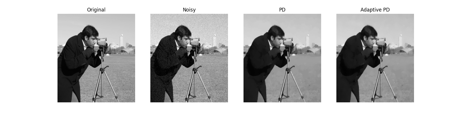
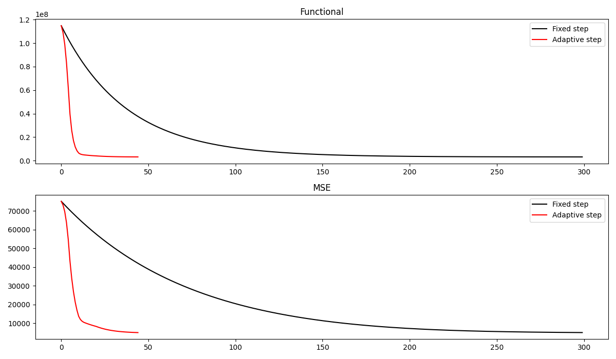
And the convergence curves of the two algorithms. We can see how the adaptive Primal-Dual produces a better estimate of the clean image in a much smaller number of iterations

fig, axs = plt.subplots(2, 1, figsize=(12, 7))
axs[0].plot(cost_fixed, "k", label="Fixed step")
axs[0].plot(cost_ada, "r", label="Adaptive step")
axs[0].legend()
axs[0].set_title("Functional")
axs[1].plot(err_fixed, "k", label="Fixed step")
axs[1].plot(err_ada, "r", label="Adaptive step")
axs[1].set_title("MSE")
axs[1].legend()
plt.tight_layout()

And to conclude we display the three different step sizes involved in the solver

fig, axs = plt.subplots(3, 1, figsize=(12, 7))
axs[0].plot(steps[0], "k")
axs[0].set_title(r"$\tau^k$")
axs[1].plot(steps[1], "k")
axs[1].set_title(r"$\mu^k$")
axs[2].plot(steps[2], "k")
axs[2].set_title(r"$\alpha^k$")
plt.tight_layout()

$\tau^k$, $\mu^k$, $\alpha^k$

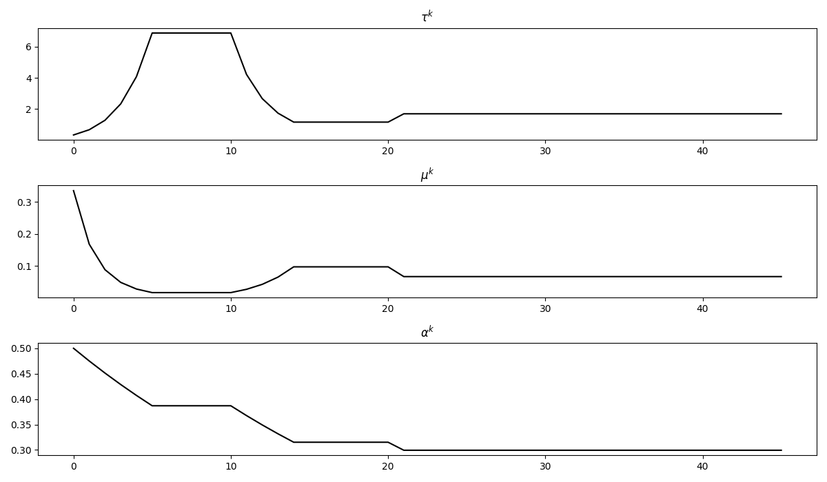
Total running time of the script: (0 minutes 10.354 seconds)

Gallery generated by Sphinx-Gallery