Note
Go to the end to download the full example code.
Regularization by Denoising (RED)
This is a follow up tutorial to the Plug and Play Priors tutorial, showcasing an competitive technical of the famous Plug-and-Play method called Regularization by Denoising (RED).
The Plug-and-Play algorithm leverges a user-defined denoiser in place of the proximal operator of the regularization term in the solution of an inverse problem, ultimately acting as an implicit prior; RED, instead, defines an the following explicit regularization term
where the dot-product of the sought after model and residual from the action of the denoiser is minimized.
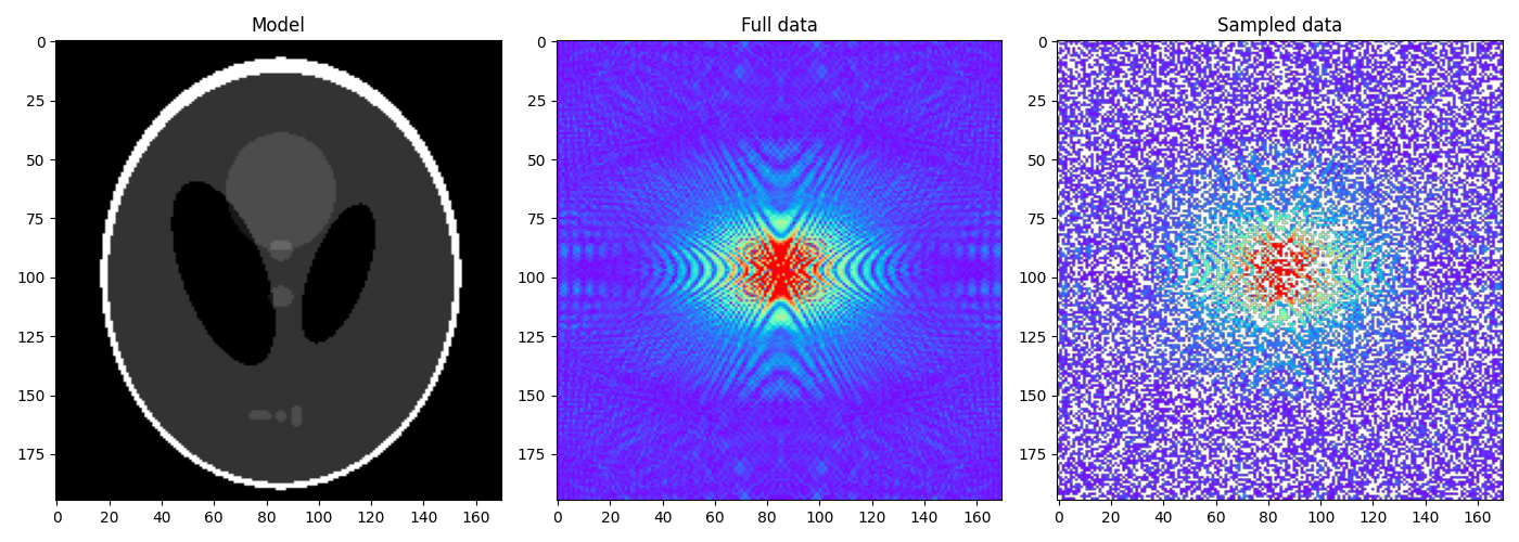
Let’s consider again a simplified MRI experiment, where the data is created by appling a 2D Fourier Transform to the input model and by randomly sampling 60% of its values, and the BM3D method as the denoiser of choice.
Two different solvers will be compared, namely:
Gradient descent, which simply uses the gradient of the data misfit term and that of the (now well defined and differentiable) regularization term;
ADMM, where the proximal of RED is solved using a fixed-point iteration.
Fixed-point method.
import bm3d
import matplotlib.pyplot as plt
import numpy as np
import pylops
from pylops.config import set_ndarray_multiplication
from pylops.utils.metrics import snr

import pyproximal

plt.close("all")
np.random.seed(0)
set_ndarray_multiplication(False)
We start by loading the famous Shepp logan phantom and creating the modelling operator
x = np.load("../testdata/shepp_logan_phantom.npy")
x = x / x.max()
ny, nx = x.shape

perc_subsampling = 0.6
nxsub = int(np.round(ny * nx * perc_subsampling))
iava = np.sort(np.random.permutation(np.arange(ny * nx))[:nxsub])
Rop = pylops.Restriction(ny * nx, iava, dtype=np.complex128)
Fop = pylops.signalprocessing.FFT2D(dims=(ny, nx))
Op = Rop * Fop
We now create and display the data alongside the model
y = Rop * Fop * x.ravel()
yfft = Fop * x.ravel()
yfft = np.fft.fftshift(yfft.reshape(ny, nx))

ymask = Rop.mask(Fop * x.ravel())
ymask = ymask.reshape(ny, nx)
ymask.data[:] = np.fft.fftshift(ymask.data)
ymask.mask[:] = np.fft.fftshift(ymask.mask)

fig, axs = plt.subplots(1, 3, figsize=(14, 5))
axs[0].imshow(x, vmin=0, vmax=1, cmap="gray")
axs[0].set_title("Model")
axs[0].axis("tight")
axs[1].imshow(np.abs(yfft), vmin=0, vmax=1, cmap="rainbow")
axs[1].set_title("Full data")
axs[1].axis("tight")
axs[2].imshow(np.abs(ymask), vmin=0, vmax=1, cmap="rainbow")
axs[2].set_title("Sampled data")
axs[2].axis("tight")
plt.tight_layout()
At this point we create a denoiser instance using the BM3D algorithm and use the gradient descent solver that we wrote at the start
def callback(x, xtrue, errhist):
    errhist.append(np.linalg.norm(x - xtrue))


def sigmad(iiter):
    return 0.1 * 0.99**iiter


# BM3D denoiser
denoiser = lambda x, sigma: bm3d.bm3d(
    np.real(x), sigma_psd=sigma, stage_arg=bm3d.BM3DStages.HARD_THRESHOLDING
)

l2 = pyproximal.proximal.L2(Op=Op, b=y.ravel())
red = pyproximal.proximal.RED(denoiser, x.shape, sigma=0.4, sigmad=sigmad, call=False)

errhistgd = []
xredgd = pyproximal.optimization.red.RED(
    l2,
    red,
    x0=np.zeros(x.size),
    solver="gradientdescent",
    alpha=0.5,
    niter=50,
    callback=lambda xx: callback(xx, x.ravel(), errhistgd),
    show=True,
)
xredgd = np.real(xredgd.reshape(x.shape))
Gradient descent algorithm
---------------------------------------------------------
Proximal operator (f): <class 'pyproximal.proximal.L2.L2'>
Proximal operator (g): <class 'pyproximal.proximal.RED.RED'>
alpha = 5.000000e-01    niter = 50

   Itn       x[0]          f
     1   1.15604e-02   2.889e+02
     2   1.17971e-02   1.144e+02
     3   6.93751e-03   5.328e+01
     4   1.03819e-03   2.824e+01
     5  -3.94497e-03   1.647e+01
     6  -9.62798e-03   1.039e+01
     7  -1.41657e-02   7.031e+00
     8  -1.66306e-02   5.090e+00
     9  -1.93065e-02   3.921e+00
    10  -2.14372e-02   3.185e+00
    11  -2.33936e-02   2.701e+00
    16  -2.90411e-02   1.694e+00
    21  -3.05927e-02   1.332e+00
    26  -2.99120e-02   1.115e+00
    31  -2.80002e-02   9.577e-01
    36  -2.56209e-02   8.203e-01
    41  -2.28929e-02   6.939e-01
    42  -2.23458e-02   6.708e-01
    43  -2.17965e-02   6.489e-01
    44  -2.12333e-02   6.282e-01
    45  -2.07053e-02   6.082e-01
    46  -2.02135e-02   5.886e-01
    47  -1.97567e-02   5.702e-01
    48  -1.93737e-02   5.529e-01
    49  -1.90143e-02   5.358e-01
    50  -1.86556e-02   5.190e-01

Total time (s) = 40.33
---------------------------------------------------------
And now we use the ADMM solver
L = np.real((Op.H * Op).eigs(neigs=1, which="LM")[0])
tau = 1.0 / L

# BM3D denoiser
denoiser = lambda x, sigma: bm3d.bm3d(
    np.real(x), sigma_psd=sigma, stage_arg=bm3d.BM3DStages.HARD_THRESHOLDING
)

# ADMM-RED
l2 = pyproximal.proximal.L2(Op=Op, b=y.ravel(), niter=10, warm=True)
red = pyproximal.proximal.RED(
    denoiser, x.shape, sigma=0.4, sigmad=sigmad, niter=5, warm=True, call=False
)

errhistadmm = []
xredadmm = pyproximal.optimization.red.RED(
    l2,
    red,
    x0=np.zeros(x.size),
    solver=pyproximal.optimization.primal.ADMM,
    tau=tau,
    niter=50,
    show=True,
    callback=lambda xx: callback(xx, x.ravel(), errhistadmm),
)[0]
xredadmm = np.real(xredadmm.reshape(x.shape))
ADMM
---------------------------------------------------------
Proximal operator (f): <class 'pyproximal.proximal.L2.L2'>
Proximal operator (g): <class 'pyproximal.proximal.RED.RED'>
tau = 1.000000e+00      niter = 50

   Itn       x[0]          f           g       J = f + g
     1   1.15604e-02   2.216e+02   0.000e+00   2.216e+02
     2   1.01482e-02   7.214e+01   0.000e+00   7.214e+01
     3   6.37155e-03   2.671e+01   0.000e+00   2.671e+01
     4   1.72745e-03   1.227e+01   0.000e+00   1.227e+01
     5  -2.77366e-03   7.000e+00   0.000e+00   7.000e+00
     6  -6.96597e-03   4.717e+00   0.000e+00   4.717e+00
     7  -1.08368e-02   3.548e+00   0.000e+00   3.548e+00
     8  -1.38539e-02   2.849e+00   0.000e+00   2.849e+00
     9  -1.60723e-02   2.397e+00   0.000e+00   2.397e+00
    10  -1.83516e-02   2.076e+00   0.000e+00   2.076e+00
    11  -2.07139e-02   1.838e+00   0.000e+00   1.838e+00
    16  -2.36279e-02   1.225e+00   0.000e+00   1.225e+00
    21  -2.13764e-02   9.796e-01   0.000e+00   9.796e-01
    26  -1.79764e-02   8.327e-01   0.000e+00   8.327e-01
    31  -1.49307e-02   7.265e-01   0.000e+00   7.265e-01
    36  -1.30449e-02   6.381e-01   0.000e+00   6.381e-01
    41  -1.07281e-02   5.530e-01   0.000e+00   5.530e-01
    42  -1.02548e-02   5.384e-01   0.000e+00   5.384e-01
    43  -9.83526e-03   5.232e-01   0.000e+00   5.232e-01
    44  -9.47296e-03   5.081e-01   0.000e+00   5.081e-01
    45  -9.05188e-03   4.935e-01   0.000e+00   4.935e-01
    46  -8.55595e-03   4.788e-01   0.000e+00   4.788e-01
    47  -8.14138e-03   4.619e-01   0.000e+00   4.619e-01
    48  -7.73302e-03   4.475e-01   0.000e+00   4.475e-01
    49  -7.40944e-03   4.343e-01   0.000e+00   4.343e-01
    50  -6.97890e-03   4.197e-01   0.000e+00   4.197e-01

Total time (s) = 203.41
---------------------------------------------------------
And finally we use the Fixed-Point solver
# BM3D
xshape = x.shape
denoiser = lambda x, sigma: bm3d.bm3d(
    x.real.reshape(xshape), sigma_psd=sigma, stage_arg=bm3d.BM3DStages.HARD_THRESHOLDING
).ravel()

# FP-RED
l2 = pyproximal.proximal.L2(Op=Op, b=y.ravel())
red = pyproximal.proximal.RED(
    denoiser, x.shape, sigma=0.4, sigmad=sigmad, niter=5, warm=True, call=False
)

errhistfp = []
xredfp = pyproximal.optimization.red.RED(
    l2,
    red,
    x0=np.zeros(x.size),
    solver="fixedpoint",
    niter=50,
    niter_inner=10,
    callback=lambda xx: callback(xx, x.ravel(), errhistfp),
    show=True,
)
xredfp = np.real(xredfp.reshape(x.shape))
Fixed point algorithm
---------------------------------------------------------
Linear Operator: <class 'pylops.linearoperator._ProductLinearOperator'>
Denoiser: <class 'pyproximal.proximal.RED._Denoise'>
sigmad = multi  sigmaOp = 1.000000e+00  sigma = 4.000000e-01
niter = 5.000000e+01    niter_inner = 10

   Itn       x[0]          f
     1   1.65149e-02   7.238e+01
     2   1.58588e-03   1.514e+01
     3  -1.08727e-02   5.812e+00
     4  -1.90211e-02   3.163e+00
     5  -2.38779e-02   2.113e+00
     6  -2.60946e-02   1.630e+00
     7  -2.63917e-02   1.379e+00
     8  -2.54913e-02   1.240e+00
     9  -2.41517e-02   1.157e+00
    10  -2.20587e-02   1.097e+00
    11  -2.02436e-02   1.057e+00
    16  -1.13673e-02   9.313e-01
    21  -6.26425e-03   8.372e-01
    26  -3.90205e-03   7.508e-01
    31  -2.60692e-03   6.693e-01
    36  -1.67991e-03   5.901e-01
    41  -9.28768e-04   5.168e-01
    42  -8.85834e-04   5.022e-01
    43  -9.32805e-04   4.875e-01
    44  -9.57026e-04   4.749e-01
    45  -8.09116e-04   4.610e-01
    46  -5.40856e-04   4.459e-01
    47  -4.27889e-04   4.317e-01
    48  -9.26203e-06   4.171e-01
    49   3.12335e-04   4.035e-01
    50   7.34846e-04   3.897e-01

Total time (s) = 41.66
---------------------------------------------------------
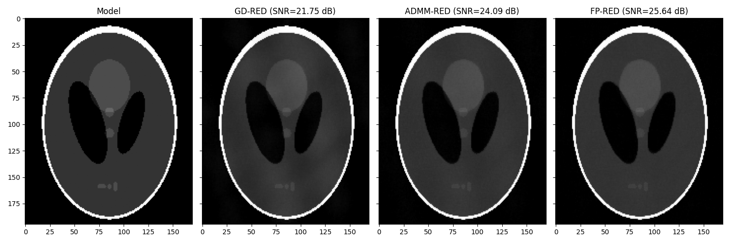
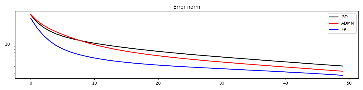
Let’s finally compare the results and the error convergence of the three variations of RED
fig, axs = plt.subplots(1, 4, sharey=True, figsize=(15, 5))
axs[0].imshow(x, vmin=0, vmax=1, cmap="gray")
axs[0].set_title("Model")
axs[0].axis("tight")
axs[1].imshow(xredgd, vmin=0, vmax=1, cmap="gray")
axs[1].set_title(f"GD-RED (SNR={snr(x, xredgd):.2f} dB)")
axs[1].axis("tight")
axs[2].imshow(xredadmm, vmin=0, vmax=1, cmap="gray")
axs[2].set_title(f"ADMM-RED (SNR={snr(x, xredadmm):.2f} dB)")
axs[2].axis("tight")
axs[3].imshow(xredfp, vmin=0, vmax=1, cmap="gray")
axs[3].set_title(f"FP-RED (SNR={snr(x, xredfp):.2f} dB)")
axs[3].axis("tight")
plt.tight_layout()

plt.figure(figsize=(12, 3))
plt.semilogy(errhistgd, "k", lw=2, label="GD")
plt.semilogy(errhistadmm, "r", lw=2, label="ADMM")
plt.semilogy(errhistfp, "b", lw=2, label="FP")

plt.title("Error norm")
plt.legend()
plt.tight_layout()
Total running time of the script: (4 minutes 46.530 seconds)